QUEUING ANALYSIS MNG 221 Management Science Queuing Analysis

QUEUING ANALYSIS MNG 221 - Management Science –

Queuing Analysis Introduction Queuing analysis is the probabilistic analysis of waiting lines. • Because time is a valuable resource, the reduction of waiting time is an important topic. • Providing quick service is an important aspect of quality customer service.

Queuing Analysis Introduction • Aware of this, more and more companies are focusing on reducing waiting time as an important component of quality improvement. • Increased service capacity will reduce waiting time and provide faster service, which usually means adding more servers.

Queuing Analysis Introduction • However, increasing service capacity has a monetary cost, and therein lies the basis of waiting line analysis: the trade-off between the cost of improved service and the cost of making customers wait.

Queuing Analysis Elements of Waiting Line Analysis

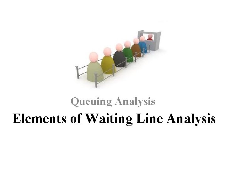
Elements of Waiting Line Analysis • Waiting lines form because people or things arrive at the servicing function, or server, faster than they can be served. • Waiting lines result because customers do not arrive at a constant, evenly paced rate, nor are they all served in an equal amount of time.

Elements of Waiting Line Analysis • Thus, a waiting line is continually increasing and decreasing in length (and is sometimes empty), and it approaches an average rate of customer arrivals and an average time to serve the customer in the long run.

Elements of Waiting Line Analysis • Decisions about waiting lines and the management of waiting lines are based on the average customer arrival and service time. • Operating Characteristics are average values for characteristics that describe the performance of a waiting line system:

Elements of Waiting Line Analysis • Example: The average time a customer must wait in line, the average number of customer waiting in line etc. NOTE: The operating characteristics of a queuing system are steady states.

Queuing Analysis The Single-Server Waiting Line System

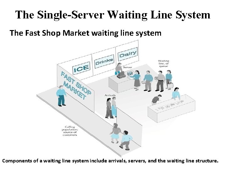
The Single-Server Waiting Line System The Fast Shop Market waiting line system Components of a waiting line system include arrivals, servers, and the waiting line structure.

The Single-Server Waiting Line System The most important factors to consider in analyzing a queuing system: 1. The Queue Discipline - is the order in which waiting customers are served. (In what order customers are served? )

The Single-Server Waiting Line System 1. The Queue Discipline Example: Customers - can be processed on a First Come, First Serve, A Predetermine Appointment, or Alphabetically according to their last name. A machine queue discipline, however can have “last-in, first-out” or “random selection”.

The Single-Server Waiting Line System The most important factors to consider in analyzing a queuing system: 2. The nature of the calling population (where customers come from). The calling population is the source of the customers, which may be finite or infinite. v Queuing systems that have an assumed infinite calling population are more common.

The Single-Server Waiting Line System The most important factors to consider in analyzing a queuing system: 3. The arrival rate (how often customers arrive at the queue). The arrival rate (λ) is the frequency at which customers arrive at a waiting line during a specified period of time according, to a probability distribution and is most frequently described by a Poisson distribution.

The Single-Server Waiting Line System The most important factors to consider in analyzing a queuing system: v. This rate can be estimated from empirical data derived from studying the system or a similar system, or it can be an average of these empirical data.

The Single-Server Waiting Line System The most important factors to consider in analyzing a queuing system: 4. The service rate (how fast customers are served). The service rate (μ) is the average number of customers who can be served during a specified time period and is often described by the negative exponential distribution.

The Single-Server Waiting Line System The most important factors to consider in analyzing a queuing system: v. A service rate is similar to an arrival rate in that it is a random variable. q. However, to analyze a queuing system, both arrivals and service must be in compatible units of measure. Thus, service time must be expressed as a service rate to correspond with an arrival rate.

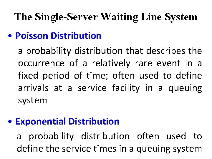
The Single-Server Waiting Line System • Poisson Distribution a probability distribution that describes the occurrence of a relatively rare event in a fixed period of time; often used to define arrivals at a service facility in a queuing system • Exponential Distribution a probability distribution often used to define the service times in a queuing system

Single-Server (SS) Model Assumptions of the basic SS Model • An infinite calling population • A first-come, first-served queue discipline • Poisson arrival rate • Exponential service times NOTE: customers must be served faster than they arrive (λ>μ) , or an infinitely large queue will build up.

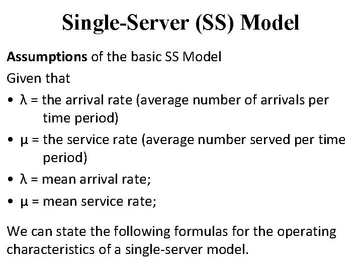
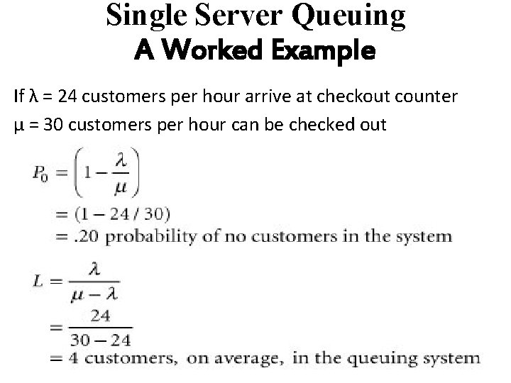
Single-Server (SS) Model Assumptions of the basic SS Model Given that • λ = the arrival rate (average number of arrivals per time period) • µ = the service rate (average number served per time period) • λ = mean arrival rate; • µ = mean service rate; We can state the following formulas for the operating characteristics of a single-server model.

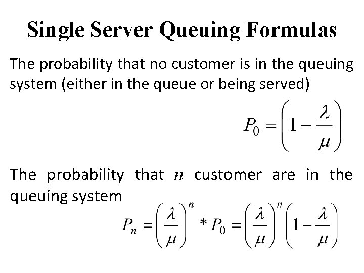
Single Server Queuing Formulas The probability that no customer is in the queuing system (either in the queue or being served) The probability that n customer are in the queuing system

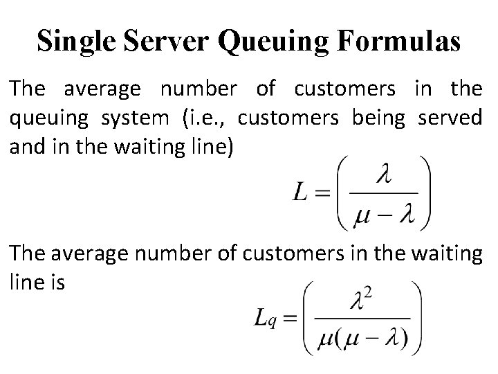
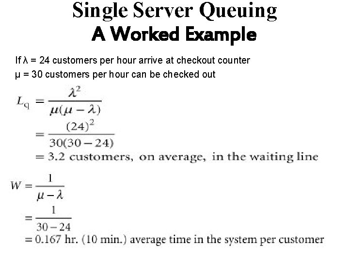
Single Server Queuing Formulas The average number of customers in the queuing system (i. e. , customers being served and in the waiting line) The average number of customers in the waiting line is

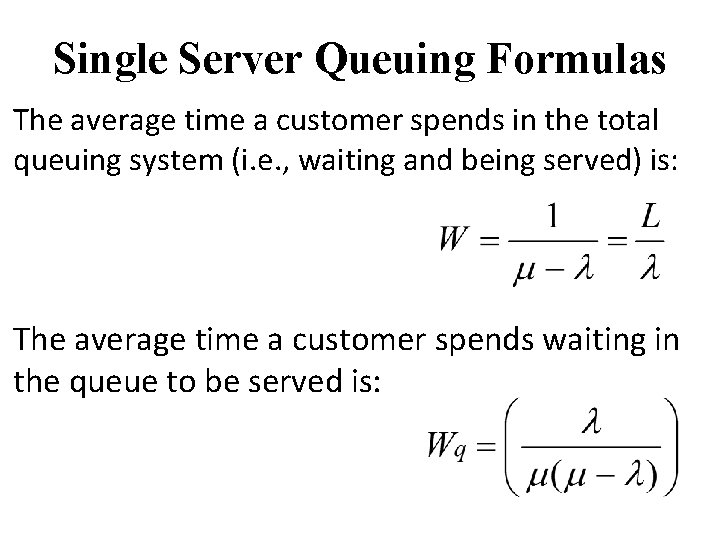
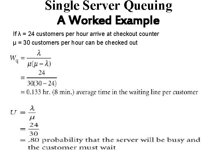
Single Server Queuing Formulas The average time a customer spends in the total queuing system (i. e. , waiting and being served) is: The average time a customer spends waiting in the queue to be served is:

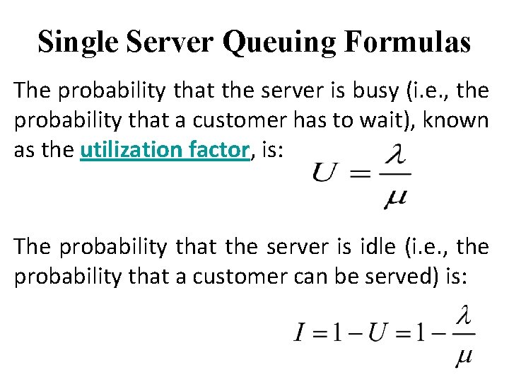
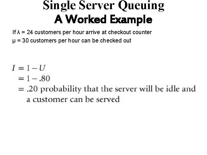
Single Server Queuing Formulas The probability that the server is busy (i. e. , the probability that a customer has to wait), known as the utilization factor, is: The probability that the server is idle (i. e. , the probability that a customer can be served) is:

Single Server Queuing Formulas • This last term, 1 - (λ /µ), is also equal to P 0. That is, the probability of no customers in the queuing system is the same as the probability that the server is idle. • We can compute these various operating characteristics for Fast Shop Market by simply substituting the average arrival and service rates into the foregoing formulas.

Queuing Analysis The Single-Server Waiting Line System A Worked Example

Single Server Queuing A Worked Example If λ = 24 customers per hour arrive at checkout counter µ = 30 customers per hour can be checked out

Single Server Queuing A Worked Example If λ = 24 customers per hour arrive at checkout counter µ = 30 customers per hour can be checked out

Single Server Queuing A Worked Example If λ = 24 customers per hour arrive at checkout counter µ = 30 customers per hour can be checked out

Single Server Queuing A Worked Example If λ = 24 customers per hour arrive at checkout counter µ = 30 customers per hour can be checked out

Single Server Queuing A Worked Example Important Aspects of General Model and Example • The operating characteristics are averages. • They are assumed to be steady-state averages. • Steady state is a constant average level that a system realizes after a period of time. • For a queuing system, the steady state is represented by the average operating statistics, also determined over a period of time.

Queuing Analysis The Effect of Operating Characteristics on Managerial Decisions

Effects of Operating Characteristics on Managerial Decisions • Alternative 1: The addition of an employee • Alternative 2: Addition of a new check out counter

Effects of Operating Characteristics on Managerial Decisions Alternative 1: The addition of an employee • The addition of an extra employee will cost the store manager $150 per week. • For each minute that average customer waiting time is reduced, the store avoids a loss in sales of $75 per week.

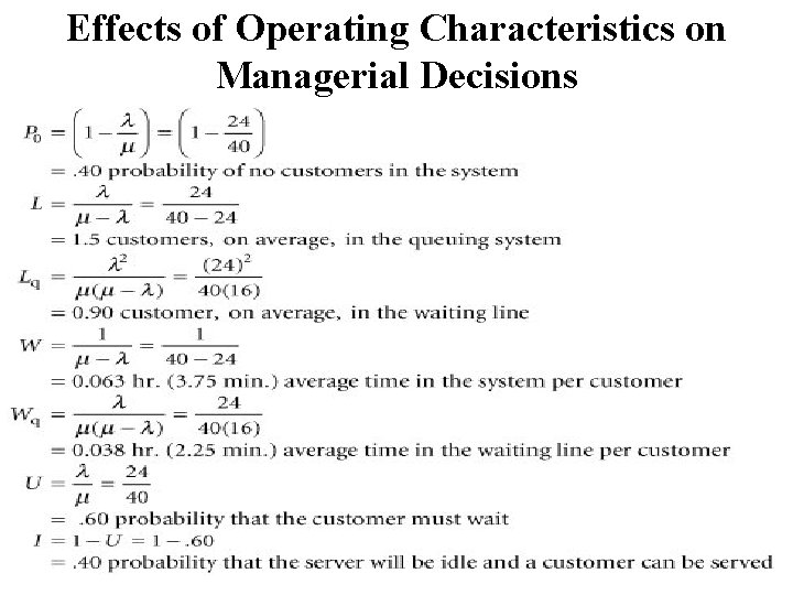
Effects of Operating Characteristics on Managerial Decisions Alternative 1: The addition of an employee • If a new employee is hired, customers can be served in less time, that is the service rate will increase to vµ = 40 customers served per hour • The arrival rate will remain the same (λ = 24 per hour) vλ = 24 customers per hour arrive at checkout counter

Effects of Operating Characteristics on Managerial Decisions

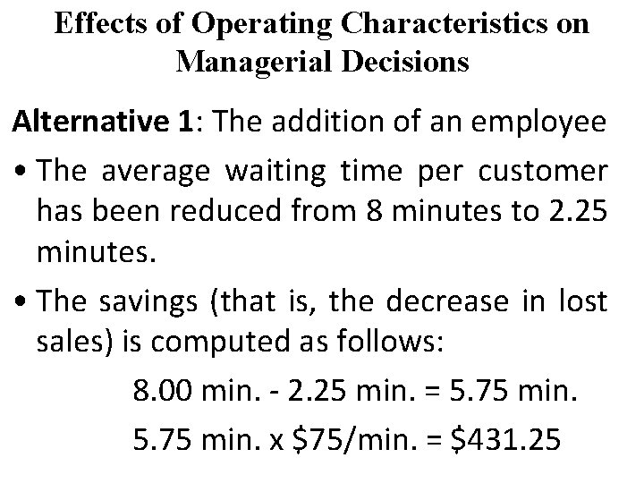
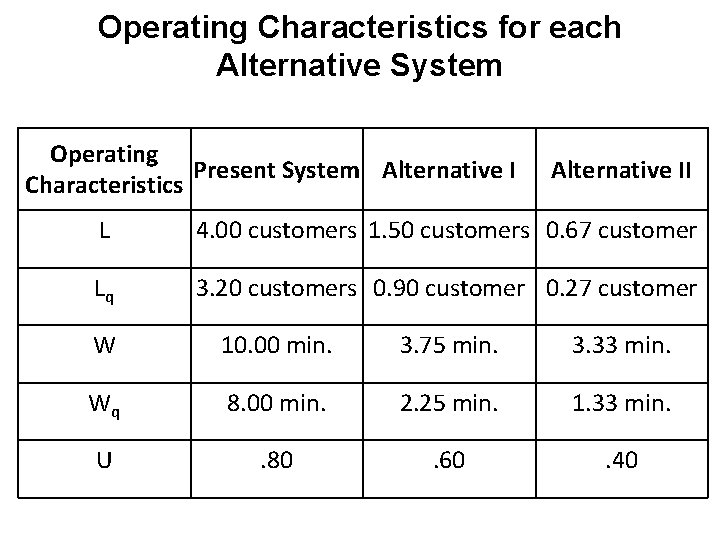
Effects of Operating Characteristics on Managerial Decisions Alternative 1: The addition of an employee • The average waiting time per customer has been reduced from 8 minutes to 2. 25 minutes. • The savings (that is, the decrease in lost sales) is computed as follows: 8. 00 min. - 2. 25 min. = 5. 75 min. x $75/min. = $431. 25

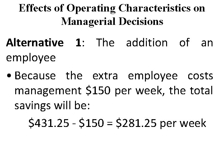
Effects of Operating Characteristics on Managerial Decisions Alternative 1: The addition of an employee • Because the extra employee costs management $150 per week, the total savings will be: $431. 25 - $150 = $281. 25 per week

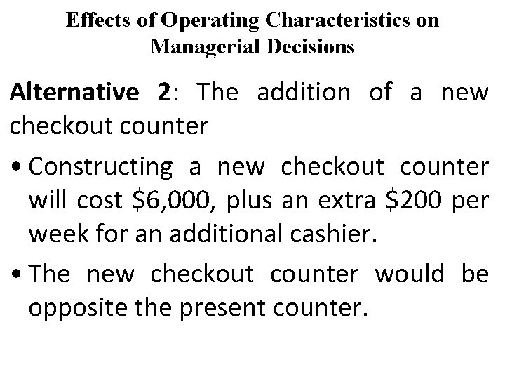
Effects of Operating Characteristics on Managerial Decisions Alternative 2: The addition of a new checkout counter • Constructing a new checkout counter will cost $6, 000, plus an extra $200 per week for an additional cashier. • The new checkout counter would be opposite the present counter.

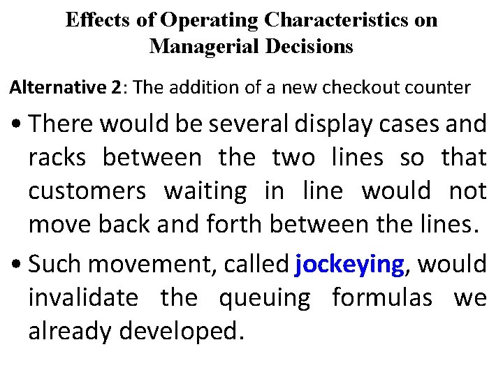
Effects of Operating Characteristics on Managerial Decisions Alternative 2: The addition of a new checkout counter • There would be several display cases and racks between the two lines so that customers waiting in line would not move back and forth between the lines. • Such movement, called jockeying, would invalidate the queuing formulas we already developed.

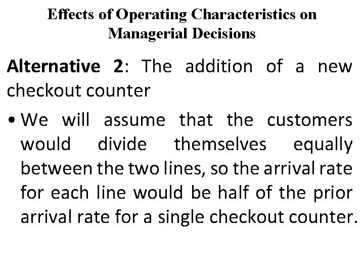
Effects of Operating Characteristics on Managerial Decisions Alternative 2: The addition of a new checkout counter • We will assume that the customers would divide themselves equally between the two lines, so the arrival rate for each line would be half of the prior arrival rate for a single checkout counter.

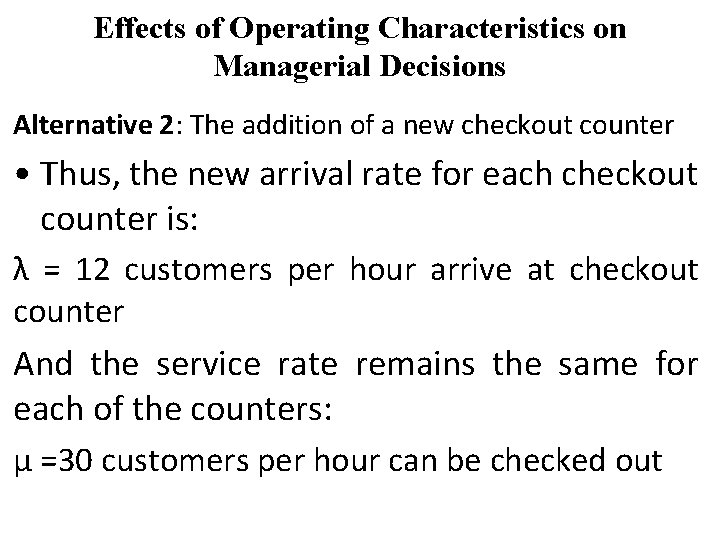
Effects of Operating Characteristics on Managerial Decisions Alternative 2: The addition of a new checkout counter • Thus, the new arrival rate for each checkout counter is: λ = 12 customers per hour arrive at checkout counter And the service rate remains the same for each of the counters: µ =30 customers per hour can be checked out

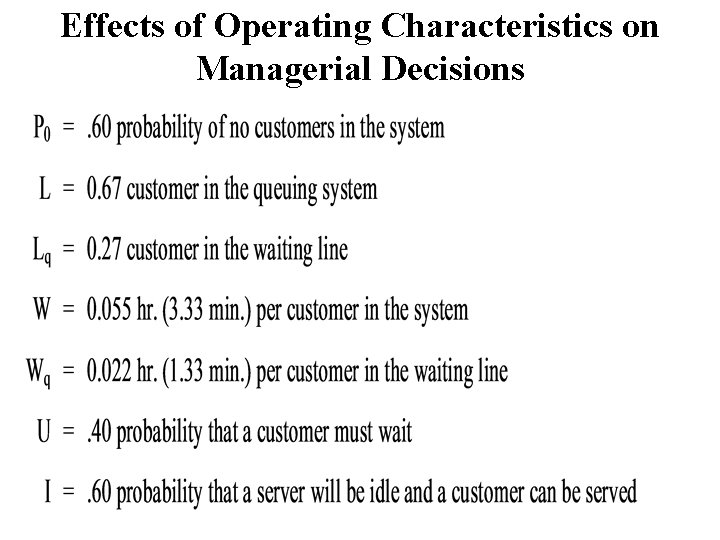
Effects of Operating Characteristics on Managerial Decisions

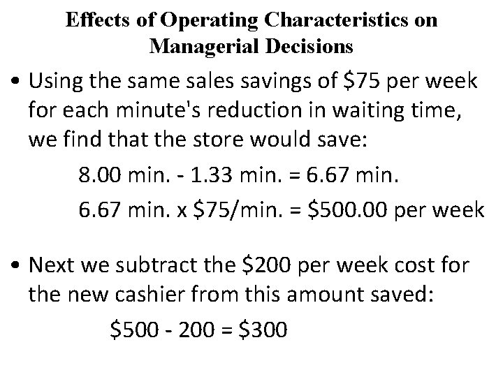
Effects of Operating Characteristics on Managerial Decisions • Using the same sales savings of $75 per week for each minute's reduction in waiting time, we find that the store would save: 8. 00 min. - 1. 33 min. = 6. 67 min. x $75/min. = $500. 00 per week • Next we subtract the $200 per week cost for the new cashier from this amount saved: $500 - 200 = $300

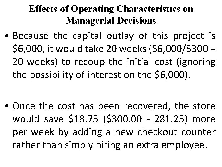
Effects of Operating Characteristics on Managerial Decisions • Because the capital outlay of this project is $6, 000, it would take 20 weeks ($6, 000/$300 = 20 weeks) to recoup the initial cost (ignoring the possibility of interest on the $6, 000). • Once the cost has been recovered, the store would save $18. 75 ($300. 00 - 281. 25) more per week by adding a new checkout counter rather than simply hiring an extra employee.

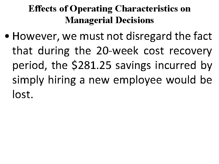
Effects of Operating Characteristics on Managerial Decisions • However, we must not disregard the fact that during the 20 -week cost recovery period, the $281. 25 savings incurred by simply hiring a new employee would be lost.

Operating Characteristics for each Alternative System Operating Present System Alternative I Characteristics Alternative II L 4. 00 customers 1. 50 customers 0. 67 customer Lq 3. 20 customers 0. 90 customer 0. 27 customer W 10. 00 min. 3. 75 min. 3. 33 min. Wq 8. 00 min. 2. 25 min. 1. 33 min. U . 80 . 60 . 40

Queuing Analysis Undefined and Constant Service Times

Single-Server (SS) Model Assumptions of the basic SS Model • An infinite calling population • A first-come, first-served queue discipline • Poisson arrival rate • Exponential service times NOTE: customers must be served faster than they arrive (λ>μ) , or an infinitely large queue will build up.

Single-Server (SS) Model Assumptions of the basic SS Model Given that • λ = the arrival rate (average number of arrivals per time period) • µ = the service rate (average number served per time period) • λ = mean arrival rate; • µ = mean service rate; We can state the following formulas for the operating characteristics of a single-server model.

Undefined and Constant Service Times • Constant service times occur with machinery and automated equipment. • Constant service times are a special case of the single-server model with general, or undefined service times.

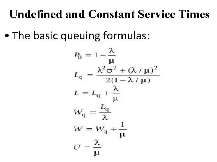
Undefined and Constant Service Times • The basic queuing formulas:

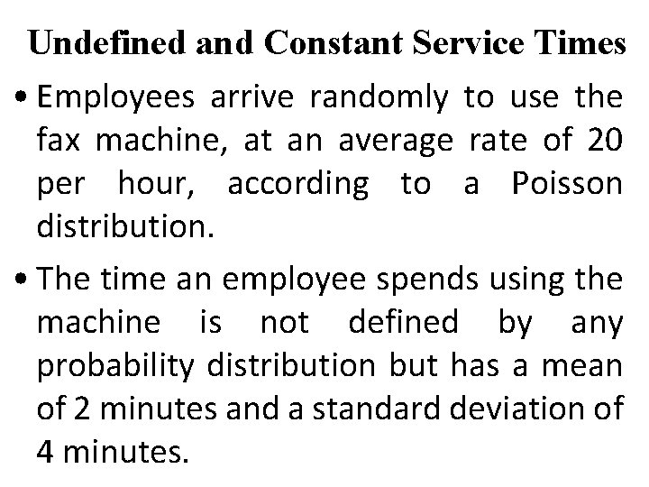
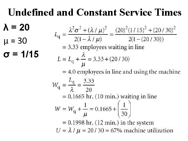
Undefined and Constant Service Times • Employees arrive randomly to use the fax machine, at an average rate of 20 per hour, according to a Poisson distribution. • The time an employee spends using the machine is not defined by any probability distribution but has a mean of 2 minutes and a standard deviation of 4 minutes.

Undefined and Constant Service Times λ = 20 µ = 30 σ = 1/15

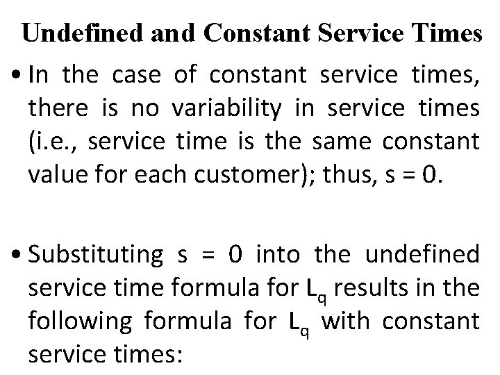
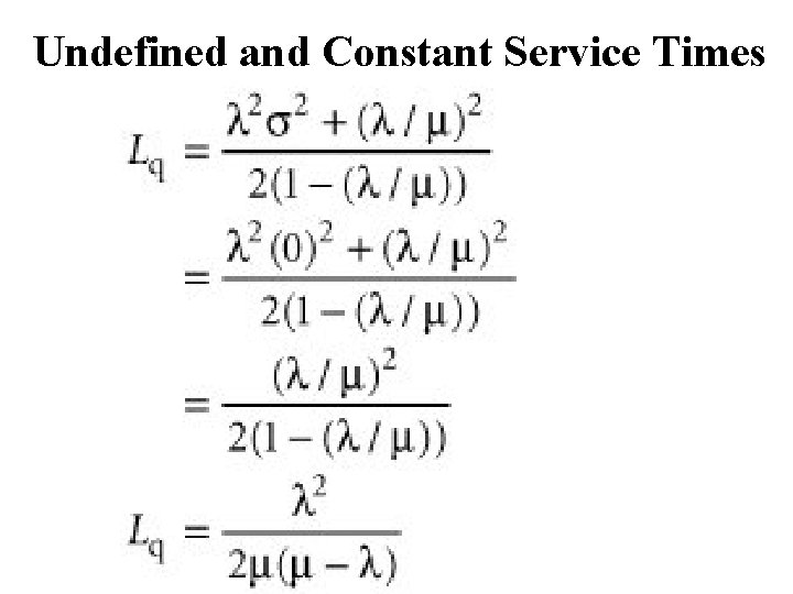
Undefined and Constant Service Times • In the case of constant service times, there is no variability in service times (i. e. , service time is the same constant value for each customer); thus, s = 0. • Substituting s = 0 into the undefined service time formula for Lq results in the following formula for Lq with constant service times:

Undefined and Constant Service Times

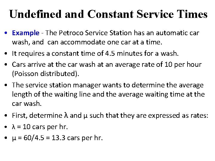
Undefined and Constant Service Times • Example - The Petroco Service Station has an automatic car wash, and can accommodate one car at a time. • It requires a constant time of 4. 5 minutes for a wash. • Cars arrive at the car wash at an average rate of 10 per hour (Poisson distributed). • The service station manager wants to determine the average length of the waiting line and the average waiting time at the car wash. • First, determine λ and µ such that they are expressed as rates: • λ = 10 cars per hr. • µ = 60/4. 5 = 13. 3 cars per hr.

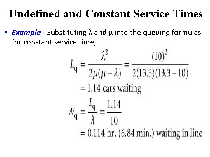
Undefined and Constant Service Times • Example - Substituting λ and µ into the queuing formulas for constant service time,

Queuing Analysis Finite Queue Length

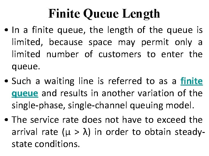
Finite Queue Length • In a finite queue, the length of the queue is limited, because space may permit only a limited number of customers to enter the queue. • Such a waiting line is referred to as a finite queue and results in another variation of the single-phase, single-channel queuing model. • The service rate does not have to exceed the arrival rate (µ > λ) in order to obtain steadystate conditions.

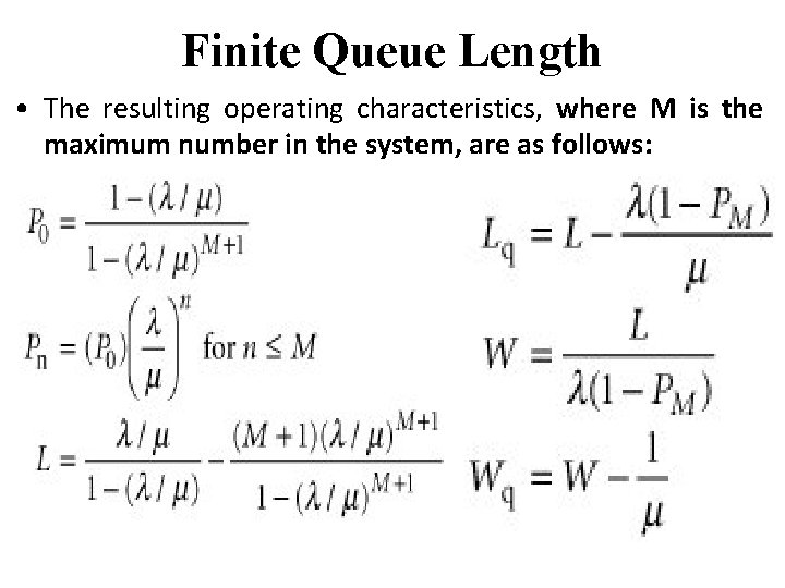
Finite Queue Length • The resulting operating characteristics, where M is the maximum number in the system, are as follows:

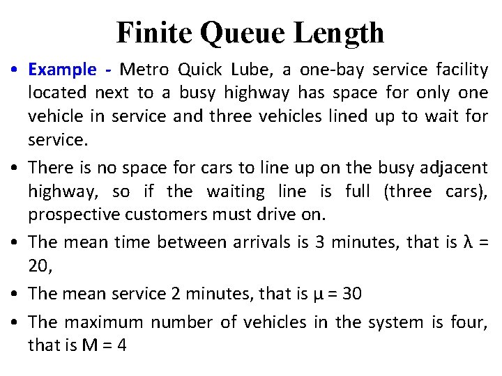
Finite Queue Length • Example - Metro Quick Lube, a one-bay service facility located next to a busy highway has space for only one vehicle in service and three vehicles lined up to wait for service. • There is no space for cars to line up on the busy adjacent highway, so if the waiting line is full (three cars), prospective customers must drive on. • The mean time between arrivals is 3 minutes, that is λ = 20, • The mean service 2 minutes, that is µ = 30 • The maximum number of vehicles in the system is four, that is M = 4

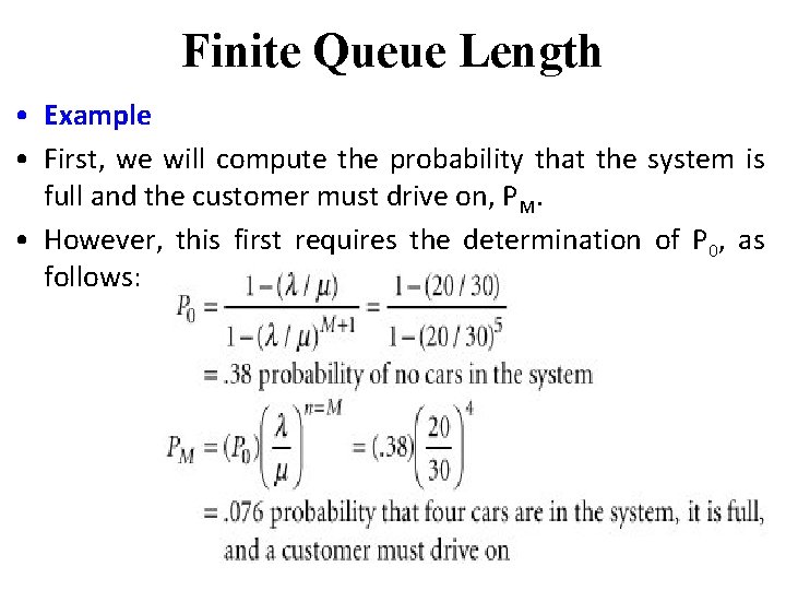
Finite Queue Length • Example • First, we will compute the probability that the system is full and the customer must drive on, PM. • However, this first requires the determination of P 0, as follows:

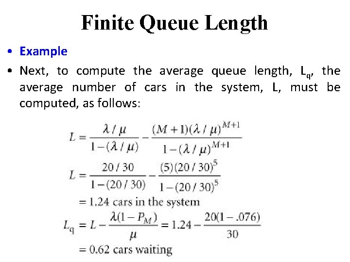
Finite Queue Length • Example • Next, to compute the average queue length, Lq, the average number of cars in the system, L, must be computed, as follows:

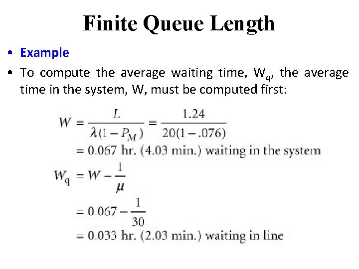
Finite Queue Length • Example • To compute the average waiting time, Wq, the average time in the system, W, must be computed first:

Queuing Analysis Finite Calling Population

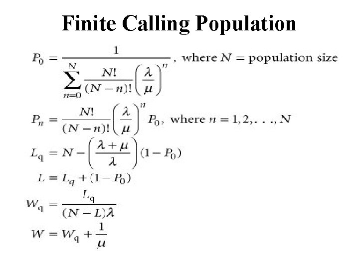
Finite Calling Population • For some waiting line systems there is a specific, limited number of potential customers that can arrive at the service facility. This is referred to as a finite calling population. • A finite calling population has the following set of formulas for determining operating characteristics. λ in this model is the arrival rate for each member of the population:

Finite Calling Population

Finite Calling Population • Example - Wheelco Manufacturing operates a shop that includes 20 machines. When a machine breaks down, it is tagged for repair, with the date of the breakdown noted and a repair person is called. • The company has one senior repair person and an assistant, who repair the machines in the same order in which they break down (a first-in, first-out queue discipline). • Machines break down according to a Poisson distribution, and the service times are exponentially distributed.

Finite Calling Population • Example The finite calling population for this example is the 20 machines in the shop, which we will designate as N. • Each machine operates an average of 200 hours before breaking down and a repair person is called. • The average time to repair a machine is 3. 6 hours. • The company would like an analysis of machine idle time due to breakdowns to determine whether the present repair staff is sufficient

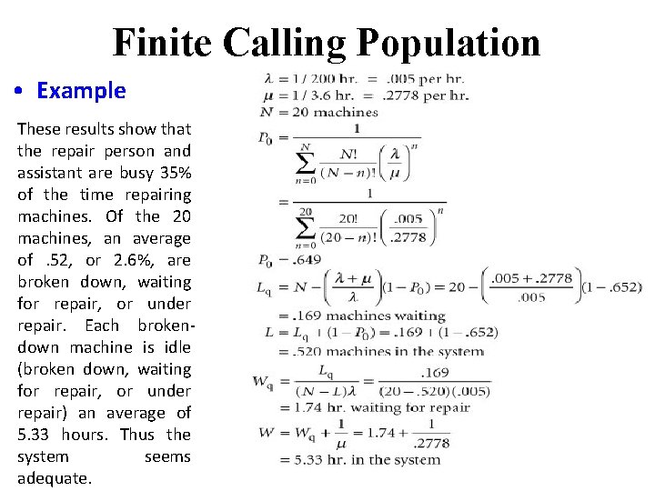
Finite Calling Population • Example These results show that the repair person and assistant are busy 35% of the time repairing machines. Of the 20 machines, an average of. 52, or 2. 6%, are broken down, waiting for repair, or under repair. Each brokendown machine is idle (broken down, waiting for repair, or under repair) an average of 5. 33 hours. Thus the system seems adequate.

Queuing Analysis Multiple-Server Waiting Line

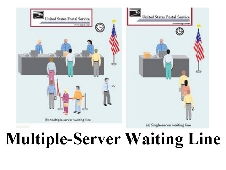
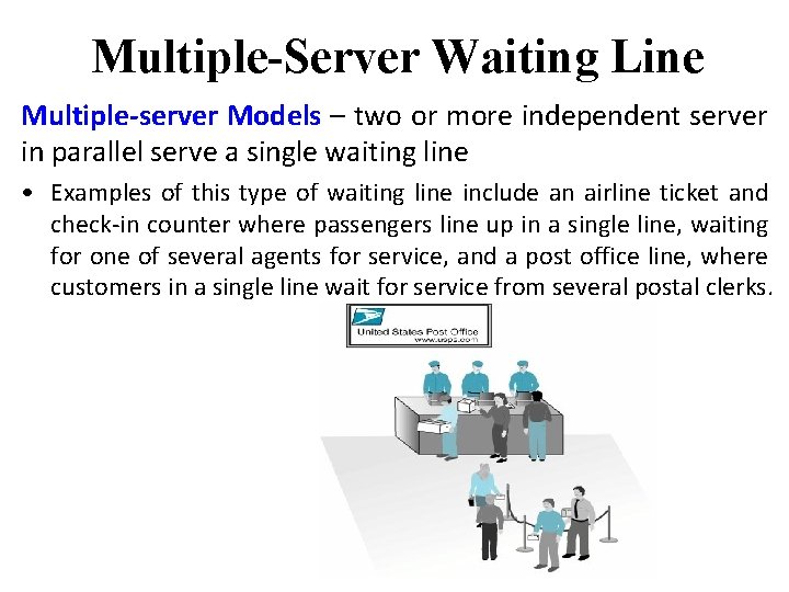
Multiple-Server Waiting Line Multiple-server Models – two or more independent server in parallel serve a single waiting line • Examples of this type of waiting line include an airline ticket and check-in counter where passengers line up in a single line, waiting for one of several agents for service, and a post office line, where customers in a single line wait for service from several postal clerks.

Multiple-Server Waiting Line • The formulas for a Multiple Server model, like single-server model formulas, have been developed on the assumption of – a first-come, first-served queue discipline, – Poisson arrivals, – exponential service times, – and an infinite calling population.

Multiple-Server Waiting Line The parameters of the multiple-server model are as follows: • λ = the arrival rate (average number of arrivals per time period) • μ = the service rate (average number served per time period) per server (channel) • c = the number of servers • cμ = the mean effective service rate for the system, which must exceed the arrival rate • cµ > λ : the total number of servers must be able to serve customers faster than they arrive.

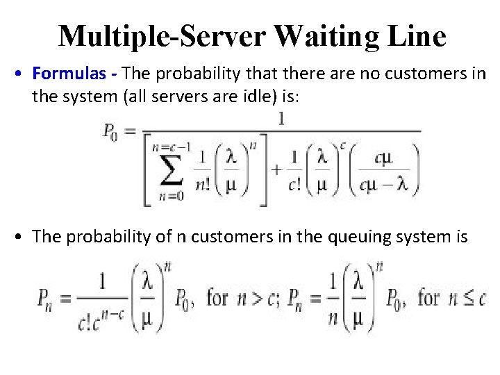
Multiple-Server Waiting Line • Formulas - The probability that there are no customers in the system (all servers are idle) is: • The probability of n customers in the queuing system is

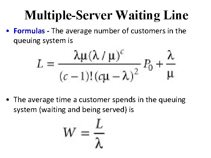
Multiple-Server Waiting Line • Formulas - The average number of customers in the queuing system is • The average time a customer spends in the queuing system (waiting and being served) is

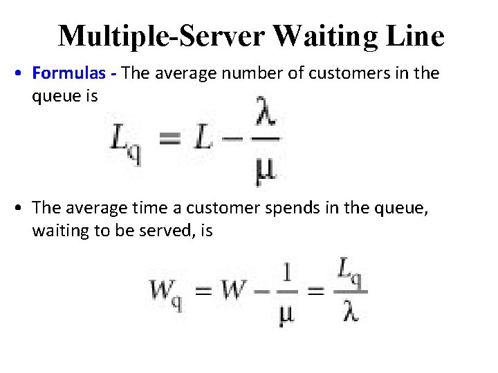
Multiple-Server Waiting Line • Formulas - The average number of customers in the queue is • The average time a customer spends in the queue, waiting to be served, is

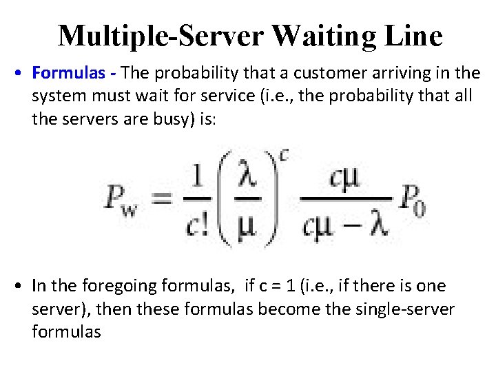
Multiple-Server Waiting Line • Formulas - The probability that a customer arriving in the system must wait for service (i. e. , the probability that all the servers are busy) is: • In the foregoing formulas, if c = 1 (i. e. , if there is one server), then these formulas become the single-server formulas

Multiple-Server Waiting Line • Example - Biggs Department Store customer service department of the store has a waiting room in which chairs are placed along the wall, in effect forming a single waiting line. • Customers come to this area with questions or complaints or to clarify matters regarding credit card bills. • The customers are served by three store representatives, each located in a partitioned stall. • Customers are served on a first-come, first-served basis. • The store management wants to analyze this queuing system because excessive waiting times can make customers angry enough to shop at other stores.

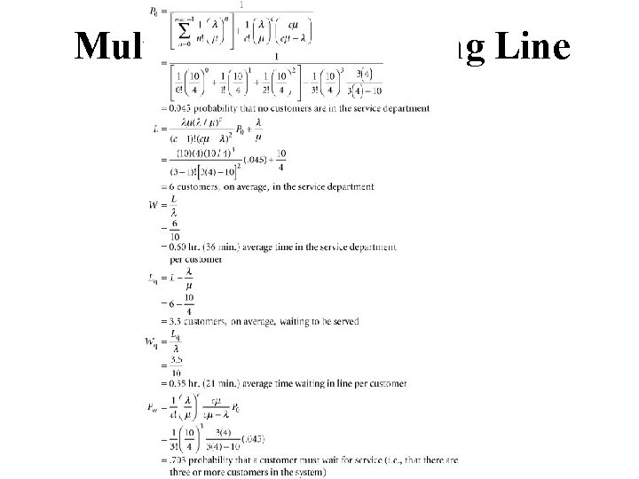
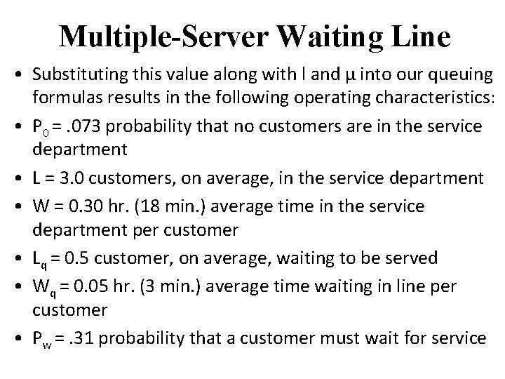
Multiple-Server Waiting Line • Example - Let us assume that a survey of the customer service department for a 12 -month period shows that the arrival rate and service rate are as follows: • λ = 10 customers per hr. arrive at the service department • µ = 4 customers per hr. can be served by each store representative • In addition, this is a three-server queuing system; therefore, • c = 3 store representatives

Multiple-Server Waiting Line

Multiple-Server Waiting Line • Substituting this value along with l and µ into our queuing formulas results in the following operating characteristics: • P 0 =. 073 probability that no customers are in the service department • L = 3. 0 customers, on average, in the service department • W = 0. 30 hr. (18 min. ) average time in the service department per customer • Lq = 0. 5 customer, on average, waiting to be served • Wq = 0. 05 hr. (3 min. ) average time waiting in line per customer • Pw =. 31 probability that a customer must wait for service