Operating Systems Advanced CPU Scheduling A Frank P

Operating Systems Advanced CPU Scheduling A. Frank - P. Weisberg

CPU Scheduling • • • 2 Basic Concepts Scheduling Criteria Simple Scheduling Algorithms Advanced Scheduling Algorithms Evaluation A. Frank - P. Weisberg

Idea of Time Quantum • Decision mode: preemptive – – a process is allowed to run until the set time slice period, called time quantum, is reached. – then a clock interrupt occurs and the running process is put on the ready queue. • How to set the quantum q? 3 A. Frank - P. Weisberg

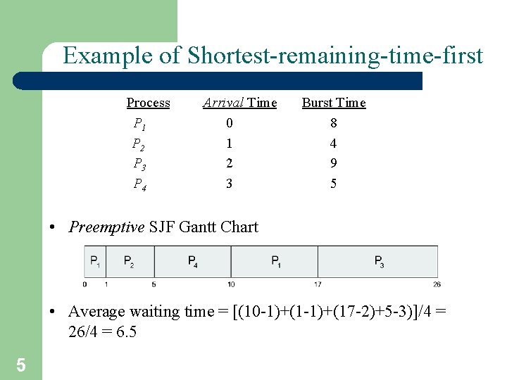
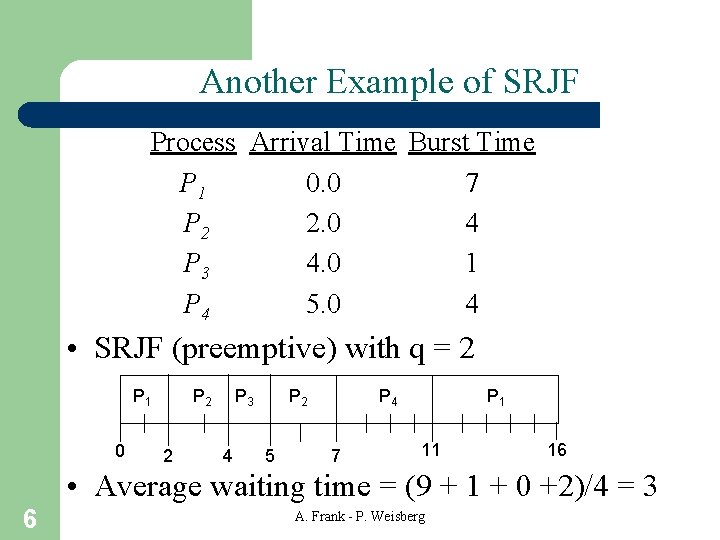
Shortest-Remaining-Job-First (SRJF) • Associate with each process the length of its next/remaining CPU burst. Use these lengths to schedule the process with the shortest time. • Preemptive – if a new process arrives with CPU burst length less than remaining time of current executing process, preempt. • Called Shortest-Remaining-Job-First (SRJF). 4 A. Frank - P. Weisberg

Example of Shortest-remaining-time-first Process. Aarri Arrival Time. T P 1 0 P 2 1 P 3 2 P 4 3 Burst Time 8 4 9 5 • Preemptive SJF Gantt Chart • Average waiting time = [(10 -1)+(17 -2)+5 -3)]/4 = 26/4 = 6. 5 5

Another Example of SRJF Process Arrival Time Burst Time P 1 0. 0 7 P 2 2. 0 4 P 3 4. 0 1 P 4 5. 0 4 • SRJF (preemptive) with q = 2 P 1 0 P 2 2 P 3 4 P 2 5 P 4 7 P 1 11 16 • Average waiting time = (9 + 1 + 0 +2)/4 = 3 6 A. Frank - P. Weisberg

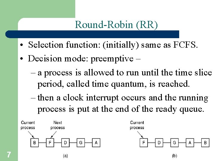
Round-Robin (RR) • Selection function: (initially) same as FCFS. • Decision mode: preemptive – – a process is allowed to run until the time slice period, called time quantum, is reached. – then a clock interrupt occurs and the running process is put at the end of the ready queue. 7 A. Frank - P. Weisberg

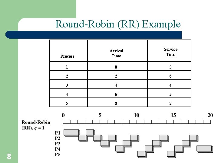
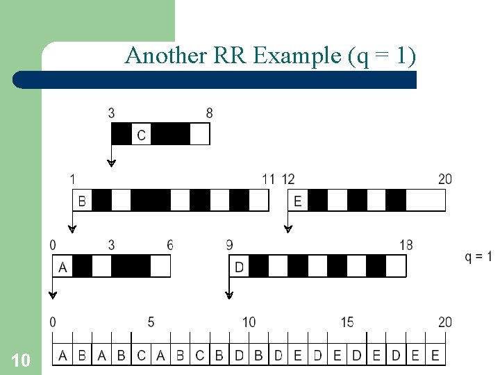
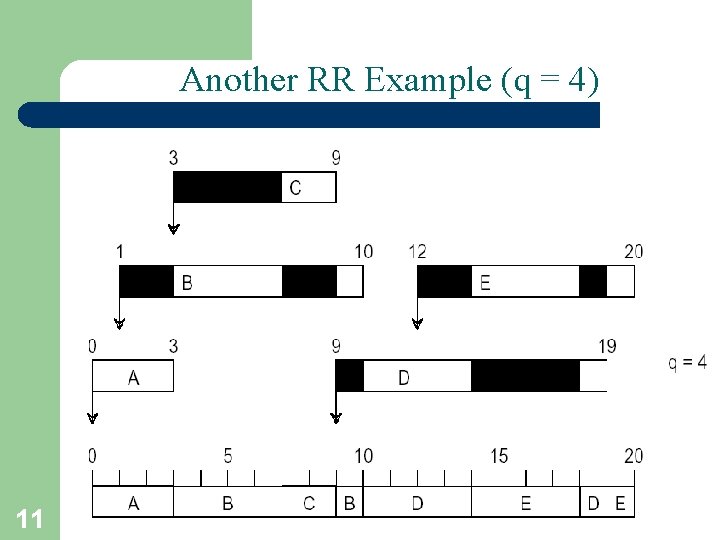
Round-Robin (RR) Example 8 Process Arrival Time Service Time 1 0 3 2 2 6 3 4 4 4 6 5 5 8 2 A. Frank - P. Weisberg

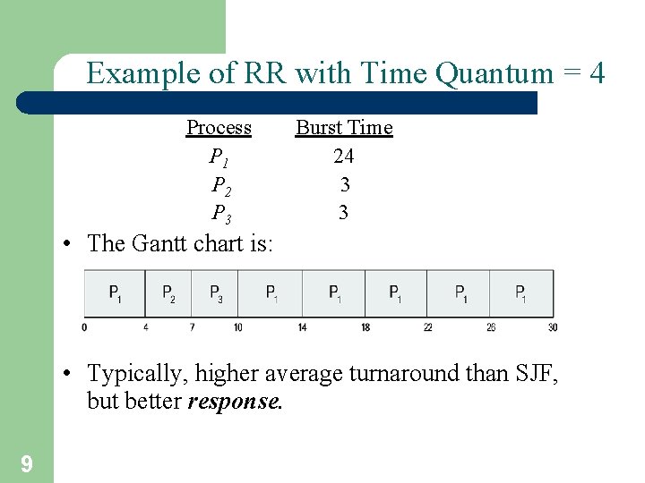
Example of RR with Time Quantum = 4 Process P 1 P 2 P 3 Burst Time 24 3 3 • The Gantt chart is: • Typically, higher average turnaround than SJF, but better response. 9

Another RR Example (q = 1) 10 A. Frank - P. Weisberg

Another RR Example (q = 4) 11 A. Frank - P. Weisberg

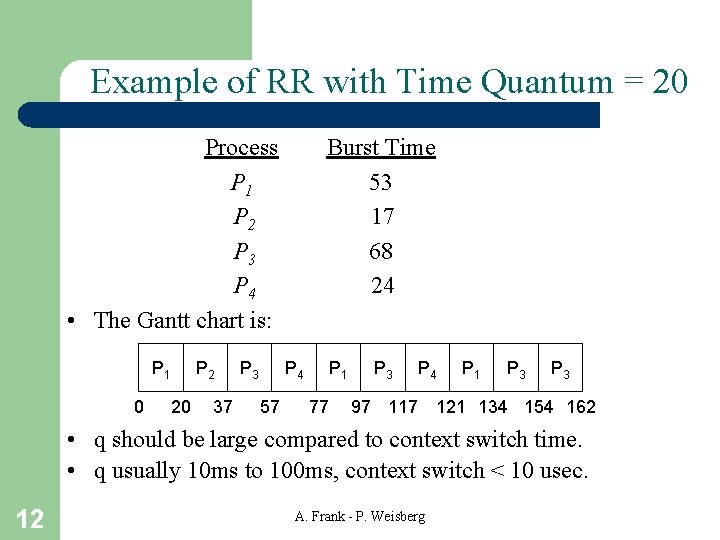
Example of RR with Time Quantum = 20 Process P 1 P 2 P 3 P 4 • The Gantt chart is: P 1 0 P 2 20 37 P 3 Burst Time 53 17 68 24 P 4 57 P 1 77 P 3 P 4 P 1 P 3 97 117 121 134 154 162 • q should be large compared to context switch time. • q usually 10 ms to 100 ms, context switch < 10 usec. 12 A. Frank - P. Weisberg

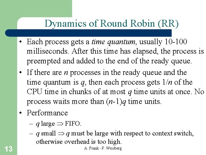
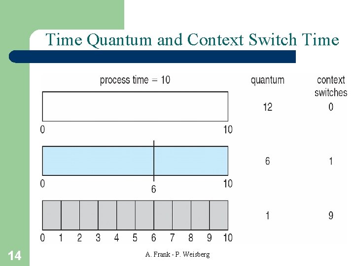
Dynamics of Round Robin (RR) • Each process gets a time quantum, usually 10 -100 milliseconds. After this time has elapsed, the process is preempted and added to the end of the ready queue. • If there are n processes in the ready queue and the time quantum is q, then each process gets 1/n of the CPU time in chunks of at most q time units at once. No process waits more than (n-1)q time units. • Performance 13 – q large FIFO. – q small q must be large with respect to context switch, otherwise overhead is too high. A. Frank - P. Weisberg

Time Quantum and Context Switch Time 14 A. Frank - P. Weisberg

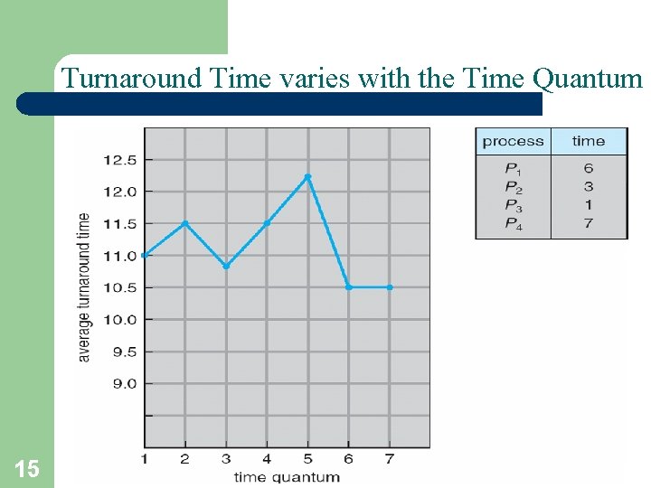
Turnaround Time varies with the Time Quantum 15 A. Frank - P. Weisberg

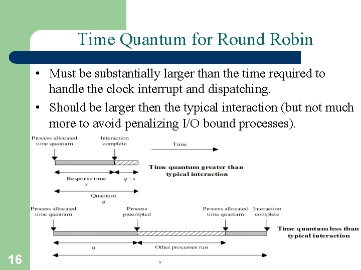
Time Quantum for Round Robin • Must be substantially larger than the time required to handle the clock interrupt and dispatching. • Should be larger then the typical interaction (but not much more to avoid penalizing I/O bound processes). 16

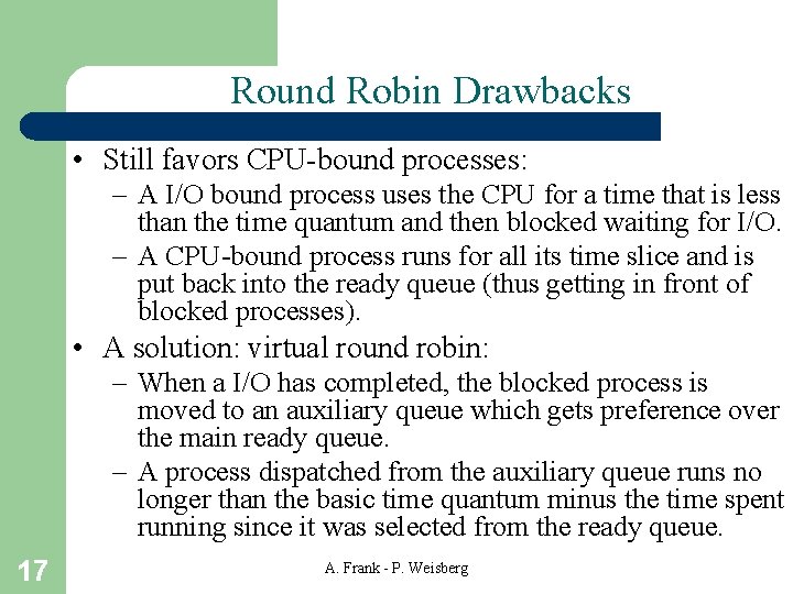
Round Robin Drawbacks • Still favors CPU-bound processes: – A I/O bound process uses the CPU for a time that is less than the time quantum and then blocked waiting for I/O. – A CPU-bound process runs for all its time slice and is put back into the ready queue (thus getting in front of blocked processes). • A solution: virtual round robin: – When a I/O has completed, the blocked process is moved to an auxiliary queue which gets preference over the main ready queue. – A process dispatched from the auxiliary queue runs no longer than the basic time quantum minus the time spent running since it was selected from the ready queue. 17 A. Frank - P. Weisberg

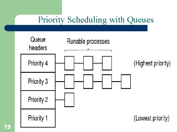
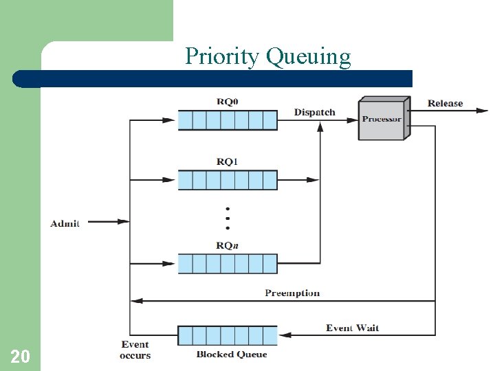
Multiple Priorities • Implemented by having multiple ready queues to represent each level of priority. • Scheduler will always choose a process of higher priority over one of lower priority. • Lower-priority may suffer starvation. • Then allow a process to change its priority based on its age or execution history. • Our first scheduling algorithms did not make use of multiple priorities. • We will now present other algorithms that use dynamic multiple priority mechanisms. 18 A. Frank - P. Weisberg

Priority Scheduling with Queues 19 A. Frank - P. Weisberg

Priority Queuing 20 A. Frank - P. Weisberg

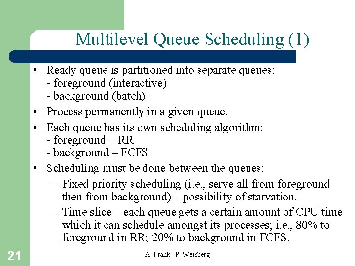
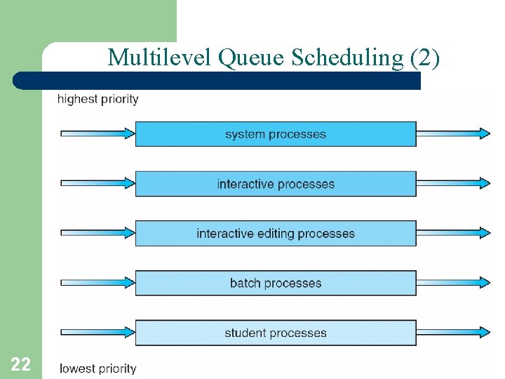
Multilevel Queue Scheduling (1) • Ready queue is partitioned into separate queues: - foreground (interactive) - background (batch) • Process permanently in a given queue. • Each queue has its own scheduling algorithm: - foreground – RR - background – FCFS • Scheduling must be done between the queues: – Fixed priority scheduling (i. e. , serve all from foreground then from background) – possibility of starvation. – Time slice – each queue gets a certain amount of CPU time which it can schedule amongst its processes; i. e. , 80% to foreground in RR; 20% to background in FCFS. 21 A. Frank - P. Weisberg

Multilevel Queue Scheduling (2) 22 A. Frank - P. Weisberg

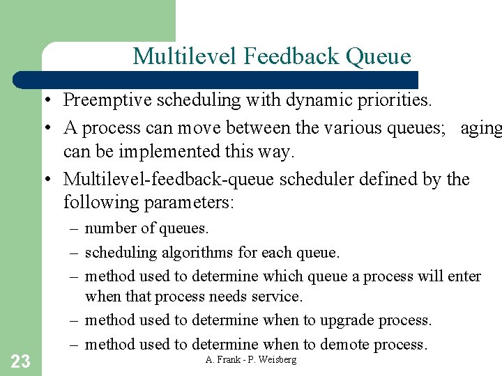
Multilevel Feedback Queue • Preemptive scheduling with dynamic priorities. • A process can move between the various queues; aging can be implemented this way. • Multilevel-feedback-queue scheduler defined by the following parameters: 23 – number of queues. – scheduling algorithms for each queue. – method used to determine which queue a process will enter when that process needs service. – method used to determine when to upgrade process. – method used to determine when to demote process. A. Frank - P. Weisberg

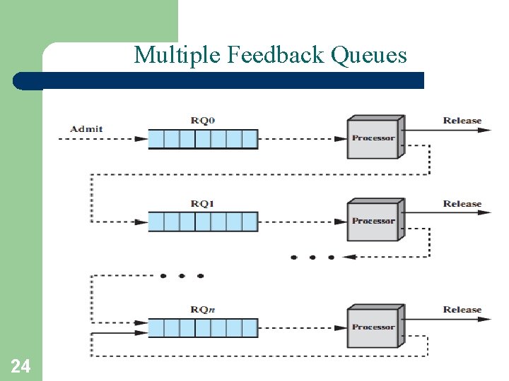
Multiple Feedback Queues 24 A. Frank - P. Weisberg

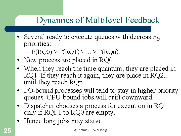
Dynamics of Multilevel Feedback • Several ready to execute queues with decreasing priorities: – P(RQ 0) > P(RQ 1) >. . . > P(RQn). • New process are placed in RQ 0. • When they reach the time quantum, they are placed in RQ 1. If they reach it again, they are place in RQ 2. . . until they reach RQn. • I/O-bound processes will tend to stay in higher priority queues. CPU-bound jobs will drift downward. • Dispatcher chooses a process for execution in RQi only if RQi-1 to RQ 0 are empty. • Hence long jobs may starve. 25 A. Frank - P. Weisberg

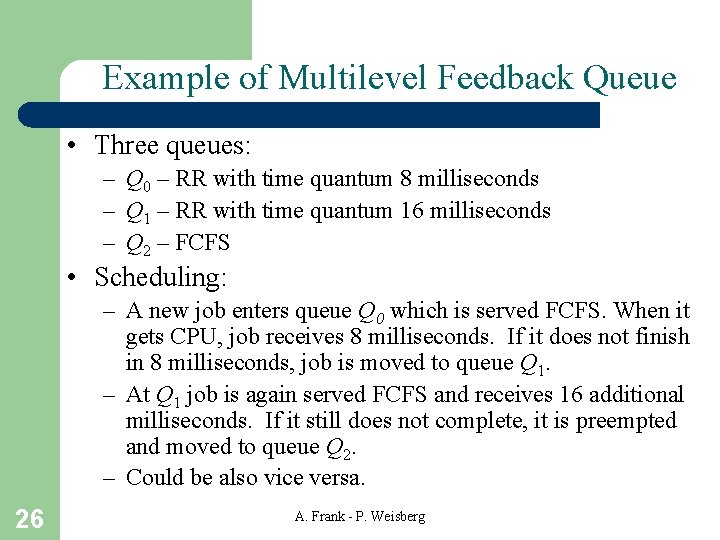
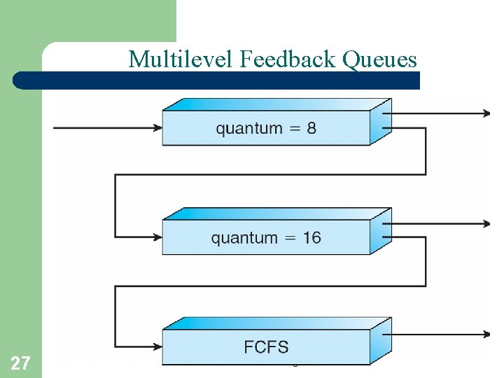
Example of Multilevel Feedback Queue • Three queues: – Q 0 – RR with time quantum 8 milliseconds – Q 1 – RR with time quantum 16 milliseconds – Q 2 – FCFS • Scheduling: – A new job enters queue Q 0 which is served FCFS. When it gets CPU, job receives 8 milliseconds. If it does not finish in 8 milliseconds, job is moved to queue Q 1. – At Q 1 job is again served FCFS and receives 16 additional milliseconds. If it still does not complete, it is preempted and moved to queue Q 2. – Could be also vice versa. 26 A. Frank - P. Weisberg

Multilevel Feedback Queues 27 A. Frank - P. Weisberg

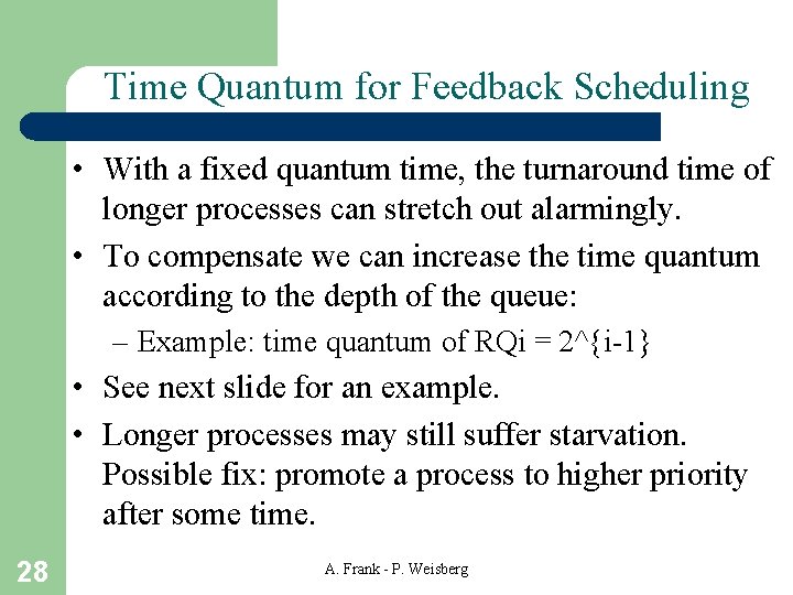
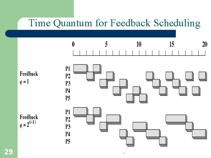
Time Quantum for Feedback Scheduling • With a fixed quantum time, the turnaround time of longer processes can stretch out alarmingly. • To compensate we can increase the time quantum according to the depth of the queue: – Example: time quantum of RQi = 2^{i-1} • See next slide for an example. • Longer processes may still suffer starvation. Possible fix: promote a process to higher priority after some time. 28 A. Frank - P. Weisberg

Time Quantum for Feedback Scheduling 29 A. Frank - P. Weisberg

Algorithms Comparison • Which one is best? • The answer depends on: – on the system workload (extremely variable). – hardware support for the dispatcher. – relative weighting of performance criteria (response time, CPU utilization, throughput. . . ). – The evaluation method used (each has its limitations. . . ). 30 • Hence the answer depends on too many factors to give any. . . A. Frank - P. Weisberg

Scheduling Algorithm Evaluation • Deterministic modeling – takes a particular predetermined workload and defines the performance of each algorithm for that workload. • Queuing models • Simulations • Implementation 31 A. Frank - P. Weisberg

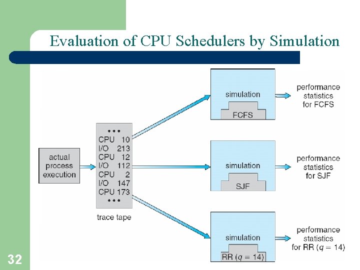
Evaluation of CPU Schedulers by Simulation 32 A. Frank - P. Weisberg

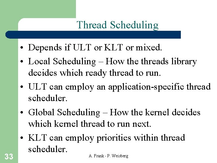
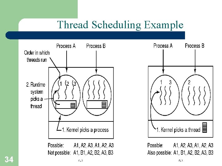
Thread Scheduling 33 • Depends if ULT or KLT or mixed. • Local Scheduling – How the threads library decides which ready thread to run. • ULT can employ an application-specific thread scheduler. • Global Scheduling – How the kernel decides which kernel thread to run next. • KLT can employ priorities within thread scheduler. A. Frank - P. Weisberg

Thread Scheduling Example 34 A. Frank - P. Weisberg