Queues and Scheduling CPU Scheduling 101 The CPU

Queues and Scheduling

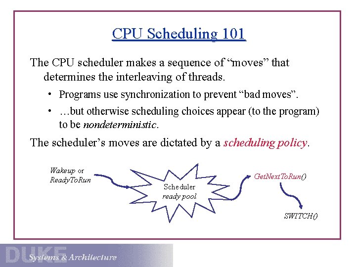
CPU Scheduling 101 The CPU scheduler makes a sequence of “moves” that determines the interleaving of threads. • Programs use synchronization to prevent “bad moves”. • …but otherwise scheduling choices appear (to the program) to be nondeterministic. The scheduler’s moves are dictated by a scheduling policy. Wakeup or Ready. To. Run Get. Next. To. Run() Scheduler ready pool SWITCH()

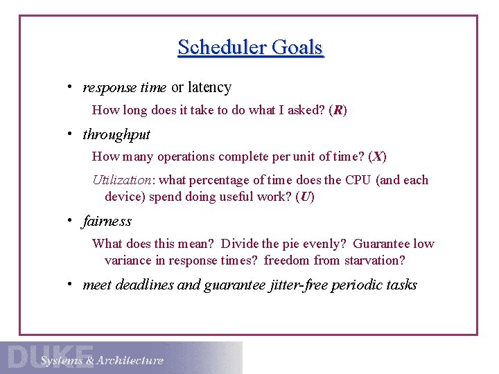
Scheduler Goals • response time or latency How long does it take to do what I asked? (R) • throughput How many operations complete per unit of time? (X) Utilization: what percentage of time does the CPU (and each device) spend doing useful work? (U) • fairness What does this mean? Divide the pie evenly? Guarantee low variance in response times? freedom from starvation? • meet deadlines and guarantee jitter-free periodic tasks

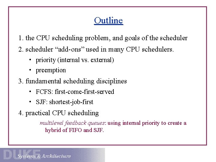
Outline 1. the CPU scheduling problem, and goals of the scheduler 2. scheduler “add-ons” used in many CPU schedulers. • priority (internal vs. external) • preemption 3. fundamental scheduling disciplines • FCFS: first-come-first-served • SJF: shortest-job-first 4. practical CPU scheduling multilevel feedback queues: using internal priority to create a hybrid of FIFO and SJF.

Priority Some goals can be met by incorporating a notion of priority into a “base” scheduling discipline. Each job in the ready pool has an associated priority value; the scheduler favors jobs with higher priority values. External priority values: • imposed on the system from outside • reflect external preferences for particular users or tasks “All jobs are equal, but some jobs are more equal than others. ” • Example: Unix nice system call to lower priority of a task. • Example: Urgent tasks in a real-time process control system.

Internal Priority Internal priority: system adjusts priority values internally as as an implementation technique within the scheduler. improve fairness, resource utilization, freedom from starvation • drop priority of jobs consuming more than their share • boost jobs that already hold resources that are in demand e. g. , internal sleep primitive in Unix kernels • boost jobs that have starved in the recent past • typically a continuous, dynamic, readjustment in response to observed conditions and events may be visible and controllable to other parts of the system

Preemption Scheduling policies may be preemptive or non-preemptive. Preemptive: scheduler may unilaterally force a task to relinquish the processor before the task blocks, yields, or completes. • timeslicing prevents jobs from monopolizing the CPU Scheduler chooses a job and runs it for a quantum of CPU time. A job executing longer than its quantum is forced to yield by scheduler code running from the clock interrupt handler. • use preemption to honor priorities Preempt a job if a higher priority job enters the ready state.

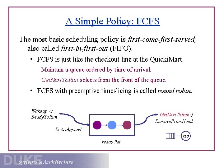
A Simple Policy: FCFS The most basic scheduling policy is first-come-first-served, also called first-in-first-out (FIFO). • FCFS is just like the checkout line at the Quicki. Mart. Maintain a queue ordered by time of arrival. Get. Next. To. Run selects from the front of the queue. • FCFS with preemptive timeslicing is called round robin. Wakeup or Ready. To. Run Get. Next. To. Run() Remove. From. Head List: : Append CPU ready list

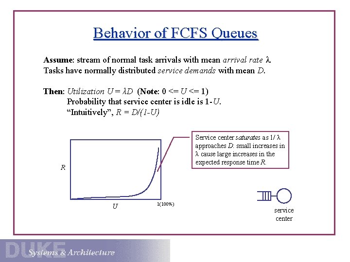
Behavior of FCFS Queues Assume: stream of normal task arrivals with mean arrival rate λ. Tasks have normally distributed service demands with mean D. Then: Utilization U = λD (Note: 0 <= U <= 1) Probability that service center is idle is 1 -U. “Intuitively”, R = D/(1 -U) Service center saturates as 1/ λ approaches D: small increases in λ cause large increases in the expected response time R. R U 1(100%) service center

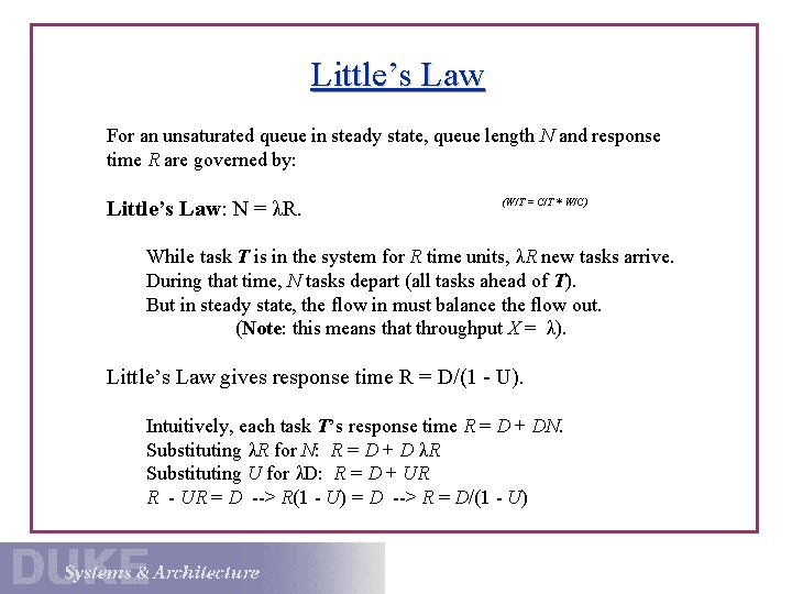
Little’s Law For an unsaturated queue in steady state, queue length N and response time R are governed by: Little’s Law: N = λR. (W/T = C/T * W/C) While task T is in the system for R time units, λR new tasks arrive. During that time, N tasks depart (all tasks ahead of T). But in steady state, the flow in must balance the flow out. (Note: this means that throughput X = λ). Little’s Law gives response time R = D/(1 - U). Intuitively, each task T’s response time R = D + DN. Substituting λR for N: R = D + D λR Substituting U for λD: R = D + UR R - UR = D --> R(1 - U) = D --> R = D/(1 - U)

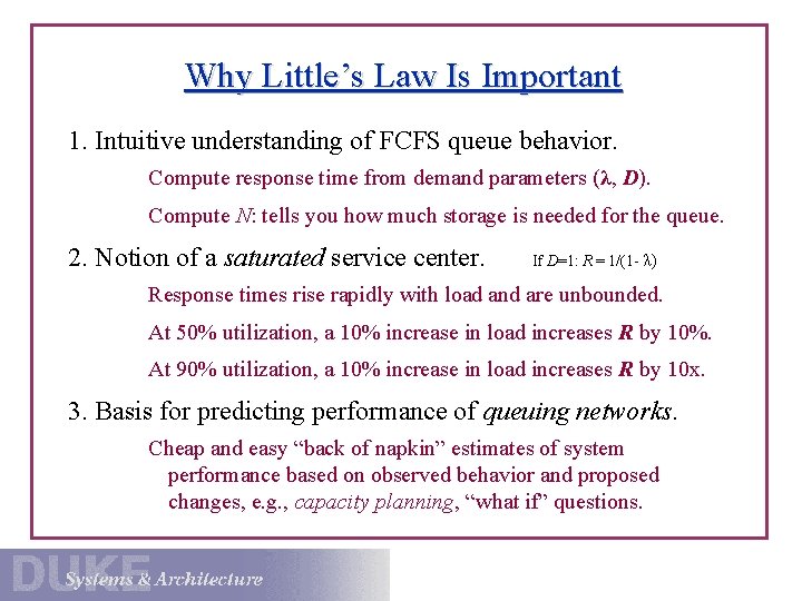
Why Little’s Law Is Important 1. Intuitive understanding of FCFS queue behavior. Compute response time from demand parameters (λ, D). Compute N: tells you how much storage is needed for the queue. 2. Notion of a saturated service center. If D=1: R = 1/(1 - λ) Response times rise rapidly with load and are unbounded. At 50% utilization, a 10% increase in load increases R by 10%. At 90% utilization, a 10% increase in load increases R by 10 x. 3. Basis for predicting performance of queuing networks. Cheap and easy “back of napkin” estimates of system performance based on observed behavior and proposed changes, e. g. , capacity planning, “what if” questions.

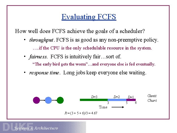
Evaluating FCFS How well does FCFS achieve the goals of a scheduler? • throughput. FCFS is as good as any non-preemptive policy. …. if the CPU is the only schedulable resource in the system. • fairness. FCFS is intuitively fair…sort of. “The early bird gets the worm”…and everyone else is fed eventually. • response time. Long jobs keep everyone else waiting. D=3 D=2 3 Time R = (3 + 5 + 6)/3 = 4. 67 D=1 5 6 Gantt Chart

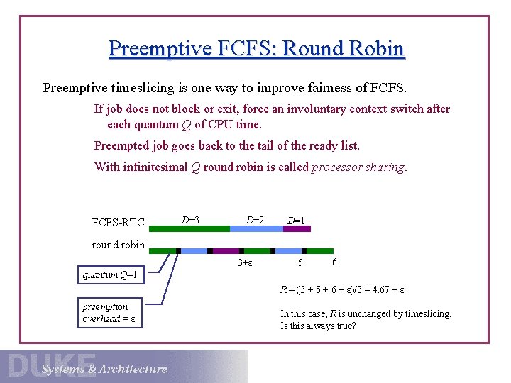
Preemptive FCFS: Round Robin Preemptive timeslicing is one way to improve fairness of FCFS. If job does not block or exit, force an involuntary context switch after each quantum Q of CPU time. Preempted job goes back to the tail of the ready list. With infinitesimal Q round robin is called processor sharing. FCFS-RTC D=3 D=2 D=1 round robin 3+ε 5 6 quantum Q=1 R = (3 + 5 + 6 + ε)/3 = 4. 67 + ε preemption overhead = ε In this case, R is unchanged by timeslicing. Is this always true?

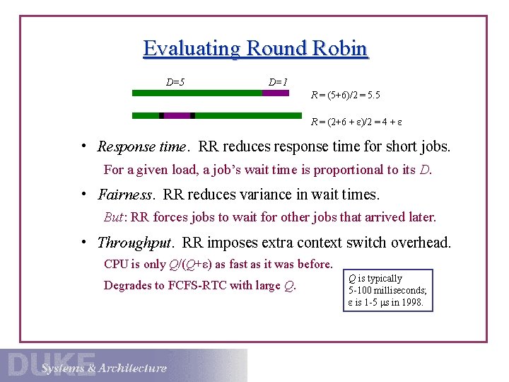
Evaluating Round Robin D=5 D=1 R = (5+6)/2 = 5. 5 R = (2+6 + ε)/2 = 4 + ε • Response time. RR reduces response time for short jobs. For a given load, a job’s wait time is proportional to its D. • Fairness. RR reduces variance in wait times. But: RR forces jobs to wait for other jobs that arrived later. • Throughput. RR imposes extra context switch overhead. CPU is only Q/(Q+ε) as fast as it was before. Degrades to FCFS-RTC with large Q. Q is typically 5 -100 milliseconds; ε is 1 -5 μs in 1998.

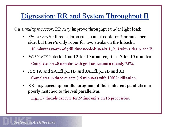
Digression: RR and System Throughput II On a multiprocessor, RR may improve throughput under light load: • The scenario: three salmon steaks must cook for 5 minutes per side, but there’s only room for two steaks on the hibachi. 30 minutes worth of grill time needed: steaks 1, 2, 3 with sides A and B. • FCFS-RTC: steaks 1 and 2 for 10 minutes, steak 3 for 10 minutes. Completes in 20 minutes with grill utilization a measly 75%. • RR: 1 A and 2 A. . . flip. . . 1 B and 3 A. . . flip. . . 2 B and 3 B. Completes in three quanta (15 minutes) with 100% utilization. • RR may speed up parallel programs if their inherent parallelism is poorly matched to the real parallelism. E. g. , 17 threads execute for N time units on 16 processors.

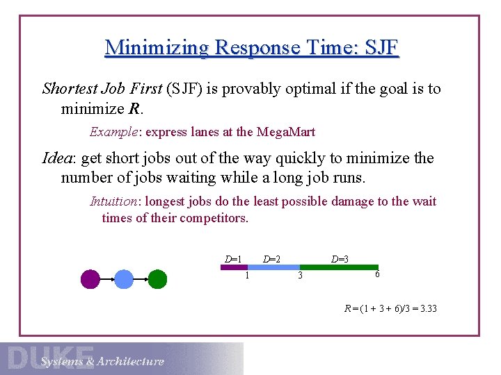
Minimizing Response Time: SJF Shortest Job First (SJF) is provably optimal if the goal is to minimize R. Example: express lanes at the Mega. Mart Idea: get short jobs out of the way quickly to minimize the number of jobs waiting while a long job runs. Intuition: longest jobs do the least possible damage to the wait times of their competitors. D=3 D=2 D=1 1 3 6 R = (1 + 3 + 6)/3 = 3. 33

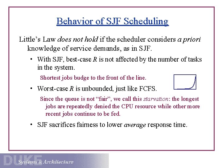
Behavior of SJF Scheduling Little’s Law does not hold if the scheduler considers a priori knowledge of service demands, as in SJF. • With SJF, best-case R is not affected by the number of tasks in the system. Shortest jobs budge to the front of the line. • Worst-case R is unbounded, just like FCFS. Since the queue is not “fair”, we call this starvation: the longest jobs are repeatedly denied the CPU resource while other more recent jobs continue to be fed. • SJF sacrifices fairness to lower average response time.

SJF in Practice Pure SJF is impractical: scheduler cannot predict D values. However, SJF has value in real systems: • Many applications execute a sequence of short CPU bursts with I/O in between. • E. g. , interactive jobs block repeatedly to accept user input. Goal: deliver the best response time to the user. • E. g. , jobs may go through periods of I/O-intensive activity. Goal: request next I/O operation ASAP to keep devices busy and deliver the best overall throughput. • Use adaptive internal priority to incorporate SJF into RR. Weather report strategy: predict future D from the recent past.

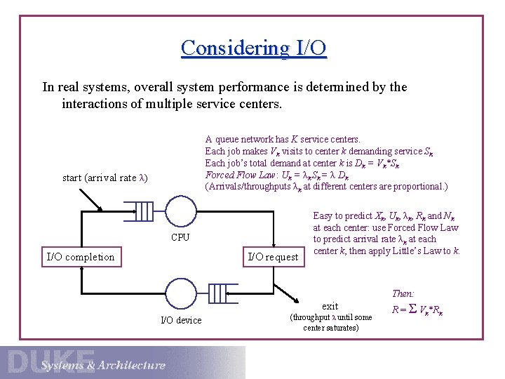
Considering I/O In real systems, overall system performance is determined by the interactions of multiple service centers. A queue network has K service centers. Each job makes Vk visits to center k demanding service Sk. Each job’s total demand at center k is Dk = Vk*Sk Forced Flow Law: Uk = λk Sk = λ Dk (Arrivals/throughputs λk at different centers are proportional. ) start (arrival rate λ) CPU I/O completion I/O request Easy to predict Xk, Uk, λk, Rk and Nk at each center: use Forced Flow Law to predict arrival rate λk at each center k, then apply Little’s Law to k. Then: exit I/O device (throughput λ until some center saturates) R = Σ Vk*Rk

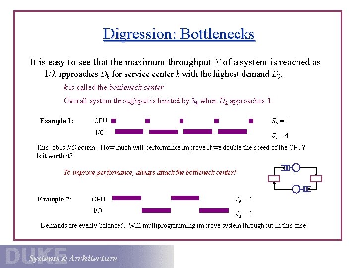
Digression: Bottlenecks It is easy to see that the maximum throughput X of a system is reached as 1/λ approaches Dk for service center k with the highest demand Dk. k is called the bottleneck center Overall system throughput is limited by λk when Uk approaches 1. Example 1: CPU S 0 = 1 I/O S 1 = 4 This job is I/O bound. How much will performance improve if we double the speed of the CPU? Is it worth it? To improve performance, always attack the bottleneck center! Example 2: CPU S 0 = 4 I/O S 1 = 4 Demands are evenly balanced. Will multiprogramming improve system throughput in this case?

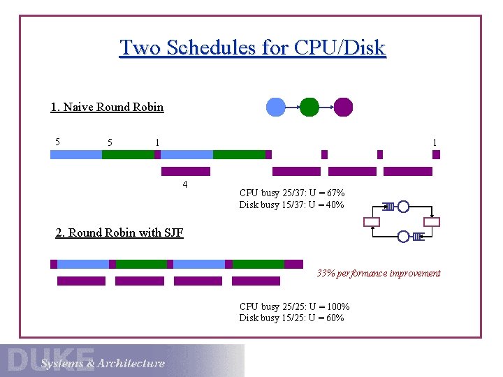
Two Schedules for CPU/Disk 1. Naive Round Robin 5 5 1 1 4 CPU busy 25/37: U = 67% Disk busy 15/37: U = 40% 2. Round Robin with SJF 33% performance improvement CPU busy 25/25: U = 100% Disk busy 15/25: U = 60%

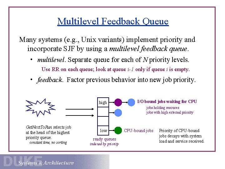
Multilevel Feedback Queue Many systems (e. g. , Unix variants) implement priority and incorporate SJF by using a multilevel feedback queue. • multilevel. Separate queue for each of N priority levels. Use RR on each queue; look at queue i-1 only if queue i is empty. • feedback. Factor previous behavior into new job priority. high I/O bound jobs waiting for CPU jobs holding resouces jobs with high external priority Get. Next. To. Run selects job at the head of the highest priority queue. constant time, no sorting low ready queues indexed by priority CPU-bound jobs Priority of CPU-bound jobs decays with system load and service received.

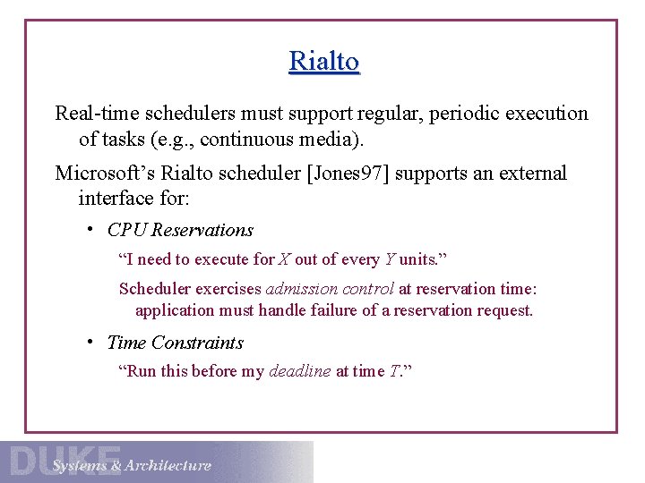
Rialto Real-time schedulers must support regular, periodic execution of tasks (e. g. , continuous media). Microsoft’s Rialto scheduler [Jones 97] supports an external interface for: • CPU Reservations “I need to execute for X out of every Y units. ” Scheduler exercises admission control at reservation time: application must handle failure of a reservation request. • Time Constraints “Run this before my deadline at time T. ”

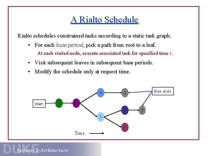
A Rialto Schedule Rialto schedules constrained tasks according to a static task graph. • For each base period, pick a path from root to a leaf. At each visited node, execute associated task for specified time t. • Visit subsequent leaves in subsequent base periods. • Modify the schedule only at request time. 4 start 3 free slots 2 1 5 Time 3

Lottery Scheduling Lottery scheduling [Waldspurger 96] is another scheduling technique. Elegant approach to periodic execution, priority, and proportional resource allocation. • Give Wp “lottery tickets” to each process p. • Get. Next. To. Run selects “winning ticket” randomly. If ΣWp = N, then each process gets CPU share Wp/N. . . probabilistically, and over a sufficiently long time interval. • Flexible: tickets are transferable to allow application-level adjustment of CPU shares. • Simple, clean, fast. Random choices are often a simple and efficient way to produce the desired overall behavior (probabilistically).