UNITII Queuing Theory Queuing Theory A mathematical method

UNIT-II Queuing Theory

Queuing Theory • A mathematical method of analyzing the congestions and delays of waiting in line. • Queuing theory examines every component of waiting in line to be served, including the arrival process, service process, number of servers, number of system places and the number of "customers" (which might be people, data packets, cars, etc. ).

Queuing Theory • It is extremely useful in predicting and evaluating system performance. • Queuing theory is used to develop more efficient queuing systems that reduce customer wait times and increase the number of customers that can be served. • Real-life applications of queuing theory include providing faster customer service, improving traffic flow, shipping orders efficiently from a warehouse and designing telecommunications systems such as call centers.

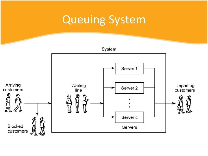
Queuing System

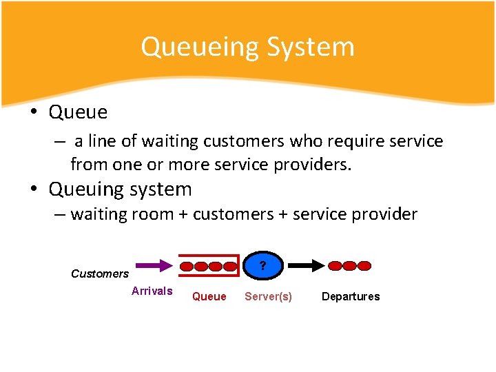
Queueing System • Queue – a line of waiting customers who require service from one or more service providers. • Queuing system – waiting room + customers + service provider ? Customers Arrivals Queue Server(s) Departures

Examples • Trucks waiting to unload or load • Workers waiting for parts • Customers waiting for products • Broken equipment waiting to be fixed • Customers waiting for service • Client systems with servers

Why Queuing Theory • Performance Measurement – Average waiting time of customer / distribution of waiting time. – Average number of customers in the system / distribution of queue length / current work backlog. – Measurement of the idle time of server / length of an idle period. – Measurement of the busy time of server / length of a busy period. – System utilization.

Characteristics of Queuing Process • Arrival Pattern of Customers – Probability distribution – Patient / impatient (balked) arrival – Stationary / nonstationary • Service Patterns – Probability distribution – State dependent / independent service – Stationary / nonstationary

Characteristics of Queuing Process (cont’d) • Queuing Disciplines – – – First come, first served (FCFS) Last come, first served (LCFS) Random selection for service (RSS) Priority queue Preemptive / non preemptive • System Capacity – Finite / infinite waiting room.

Characteristics of Queuing Process (cont’d) • Number of Service Channels – Single channel / multiple channels – Single queue / multiple queues • Stages of Service – Single stage (e. g. hair-styling salon) – Multiple stages (e. g. manufacturing process) – Process recycling or feedback

Queuing Models • In queuing theory, a queuing model is used to approximate a real queuing situation or system, so the queuing behaviour can be analysed mathematically. • Queuing systems are usually described by three values separated by slashes • Arrival distribution / service distribution / # of servers

Queuing Models • Widely used to estimate desired performance measures of the system • Provide rough estimate of a performance measure • Typical measures – Server utilization – Length of waiting lines – Delays of customers • Applications – Determine the minimum number of servers needed at a service center – Detection of performance bottleneck or congestion – Evaluate alternative system designs

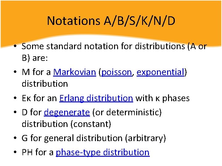
Kendall Notation A/B/S/K/N/D where: • • A is the inter arrival time distribution B is the service time distribution S is the number of servers K is the system capacity N is the calling population D is the service discipline assumed Many times the last members are omitted, so the notation becomes A/B/S and it is assumed that K = , N = and D = FIFO.

Notations A/B/S/K/N/D • Some standard notation for distributions (A or B) are: • M for a Markovian (poisson, exponential) distribution • Eκ for an Erlang distribution with κ phases • D for degenerate (or deterministic) distribution (constant) • G for general distribution (arbitrary) • PH for a phase-type distribution

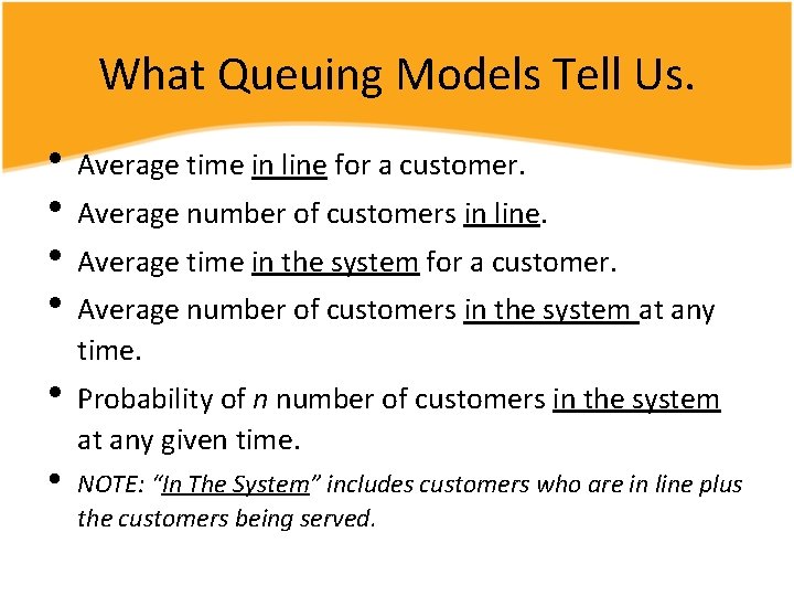
What Queuing Models Tell Us. • Average time in line for a customer. • Average number of customers in line. • Average time in the system for a customer. • Average number of customers in the system at any time. • Probability of n number of customers in the system • at any given time. NOTE: “In The System” includes customers who are in line plus the customers being served.

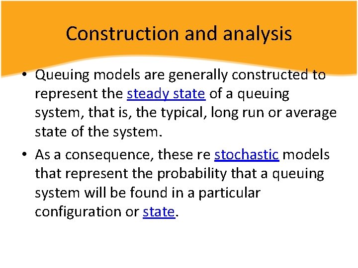
Construction and analysis • Queuing models are generally constructed to represent the steady state of a queuing system, that is, the typical, long run or average state of the system. • As a consequence, these re stochastic models that represent the probability that a queuing system will be found in a particular configuration or state.

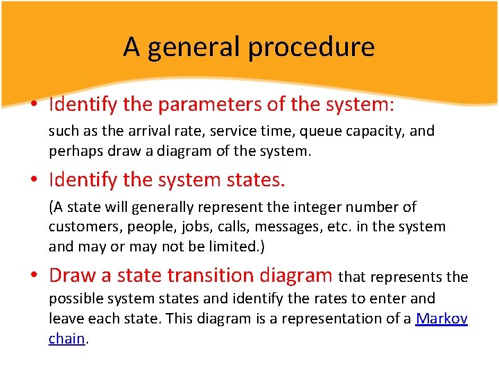
A general procedure • Identify the parameters of the system: such as the arrival rate, service time, queue capacity, and perhaps draw a diagram of the system. • Identify the system states. (A state will generally represent the integer number of customers, people, jobs, calls, messages, etc. in the system and may or may not be limited. ) • Draw a state transition diagram that represents the possible system states and identify the rates to enter and leave each state. This diagram is a representation of a Markov chain.

A general procedure(con’d) • Because the state transition diagram represents the steady state situation. • Express all the state probabilities in terms of the empty state probability, using the inter-state transition relationships. • Determine the empty state probability by using the fact that all state probabilities always sum to 1.

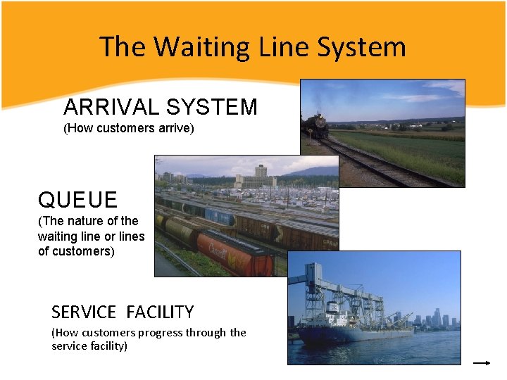
The Waiting Line System ARRIVAL SYSTEM (How customers arrive) QUEUE (The nature of the waiting line or lines of customers) SERVICE FACILITY (How customers progress through the service facility)

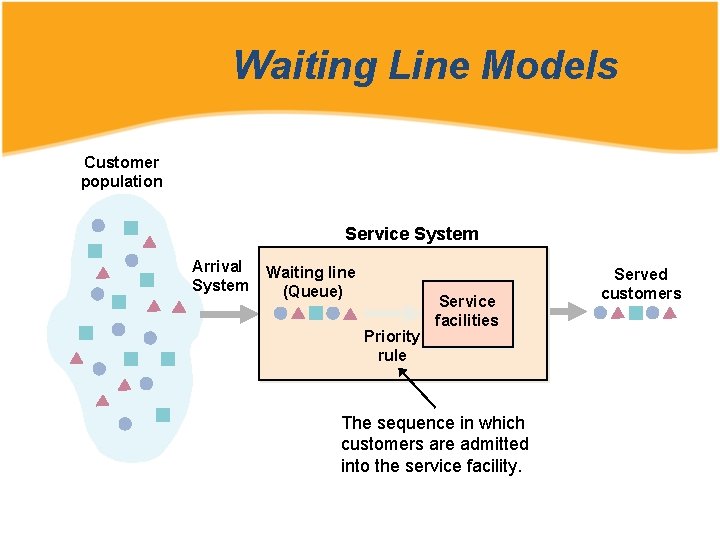
Waiting Line Models Customer population Service System Arrival System Waiting line (Queue) Priority rule Service facilities The sequence in which customers are admitted into the service facility. Served customers

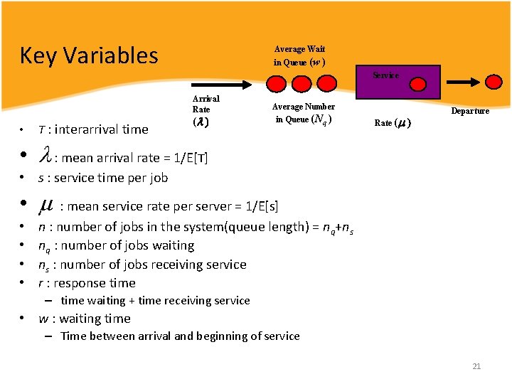
Key Variables Average Wait in Queue (w ) Service Arrival Rate • Τ : interarrival time ( Average Number in Queue (Nq ) Rate ( Departure • : mean arrival rate = 1/E[Τ] • s : service time per job • : mean service rate per server = 1/E[s] • • n : number of jobs in the system(queue length) = nq+ns nq : number of jobs waiting ns : number of jobs receiving service r : response time – time waiting + time receiving service • w : waiting time – Time between arrival and beginning of service 21

The Service Facility • Channels • How many paths (ways to get through the system) are there after getting in line? • EG: Mc. Donalds drive-thru is one channel. • Phases • How many stops must a customer make, after getting in line? (Single-phase means only one stop for service. )

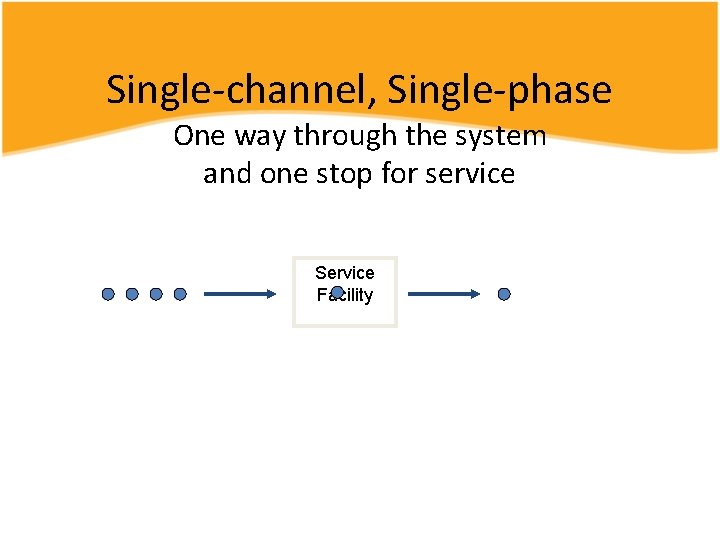
Single-channel, Single-phase One way through the system and one stop for service Service Facility

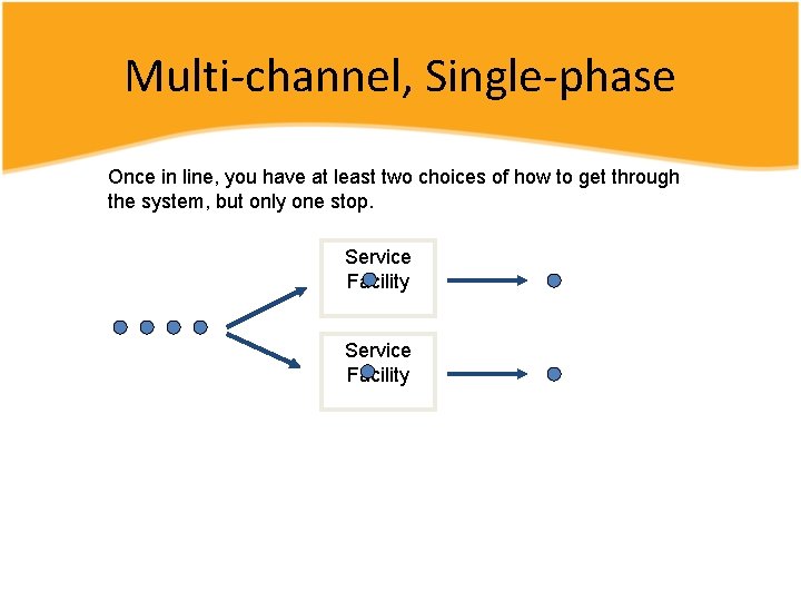
Multi-channel, Single-phase Once in line, you have at least two choices of how to get through the system, but only one stop. Service Facility

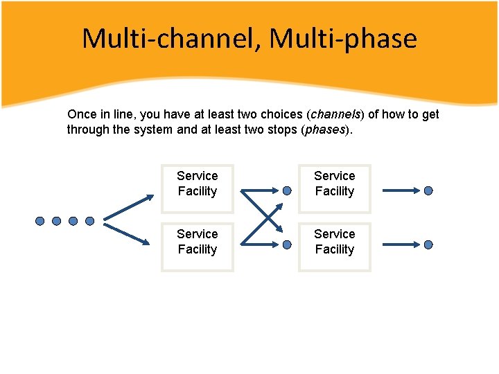
Multi-channel, Multi-phase Once in line, you have at least two choices (channels) of how to get through the system and at least two stops (phases). Service Facility

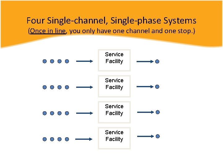
Four Single-channel, Single-phase Systems (Once in line, you only have one channel and one stop. ) Service Facility

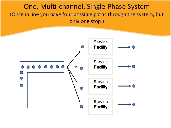
One, Multi-channel, Single-Phase System (Once in line you have four possible paths through the system, but only one stop. ) Service Facility

Example • M/M/3/20/1500/FCFS – Time between successive arrivals is exponentially distributed – Service times are exponentially distributed – Three servers – 20 buffers = 3 service + 17 waiting • After 20, all arriving jobs are lost – Total of 1500 jobs that can be serviced – Service discipline is first-come-first-served 28

Common Models • The simplest queuing model is M/M/1 • where both the arrival time and service time are exponentially distributed. • The M/D/1 model has ex po n e ntially distributed arrival times but fixed service time. • The M/M/n model has multiple servers.

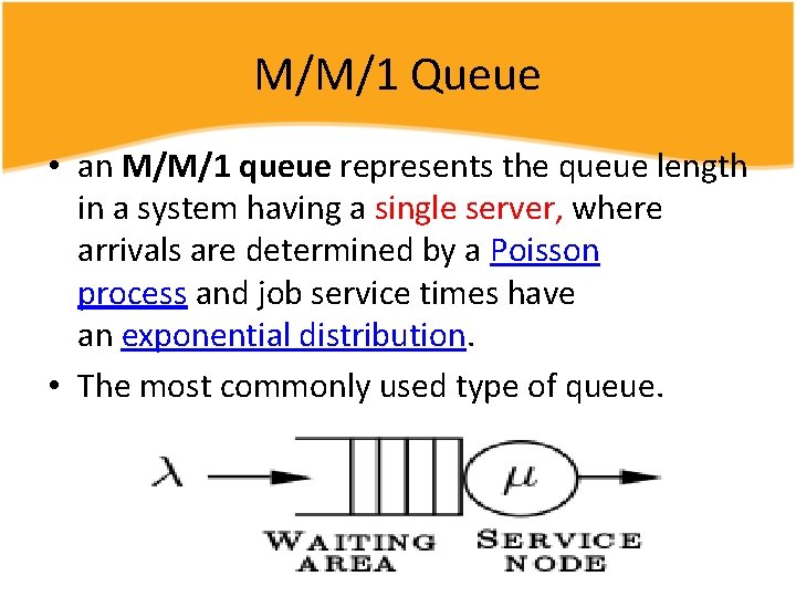
M/M/1 Queue • an M/M/1 queue represents the queue length in a system having a single server, where arrivals are determined by a Poisson process and job service times have an exponential distribution. • The most commonly used type of queue.

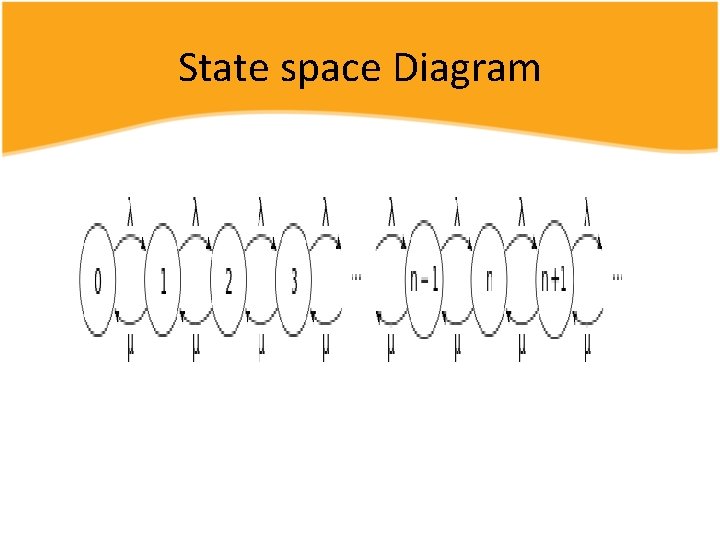
Arrival System • An M/M/1 queue is a stochastic process whose state space is the set {0, 1, 2, 3, . . . } where the value corresponds to the number of customers in the system, including any currently in service. • Arrivals occur at rate λ according to a Poisson process and move the process from state i to i + 1.

Arrival System • Arrival Populations are either… • • Limited (EG: Only people age 21 or over. ) Unlimited (EG: cars arriving at a toll booth) Arrival Patterns are either… • • Random (Each arrival is independent) Scheduled (EG: Doctor’s office visits) Behavior of the Arrivals • • • Balking (Seeing a long line and avoiding it. ) Reneging (Get tired of waiting and leave the line) Jockeying (Switching lines)

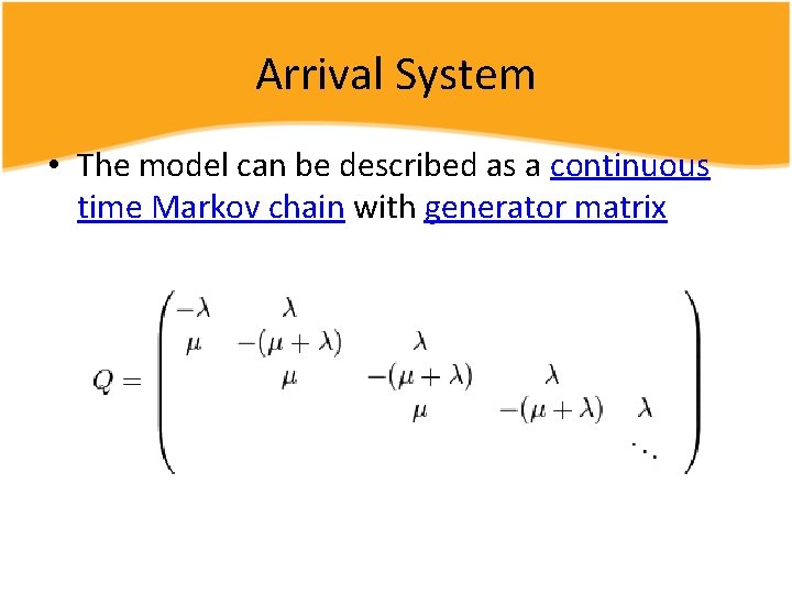
Arrival System • The model can be described as a continuous time Markov chain with generator matrix

State space Diagram

Distribution model(service) • Service times have an exponential distribution with parameter μ in the M/M/1 queue. • A single server serves customers one at a time from the front of the queue, according to a first-come, first-served discipline. When the service is complete the customer leaves the queue and the number of customers in the system reduces by one

Distribution • Distribution model – Exponential – Erlang – Hyper-exponential – General • cf. – Jobs = customers – Device = service center = queue – Buffer = waiting position 36

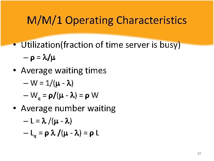
M/M/1 Operating Characteristics • Utilization(fraction of time server is busy) – ρ = / • Average waiting times – W = 1/( - ) – Wq = ρ/( - ) = ρ W • Average number waiting – L = /( - ) – Lq = ρ /( - ) = ρ L 37

Little’s formula • John Little's proof was published in 1961, Case Western Reserve University. • The result applies to any system, and particularly, it applies to systems within systems. So in a bank, the customer line might be one subsystem, and each of the tellers another subsystem, and Little's result could be applied to each one, as well as the whole thing.

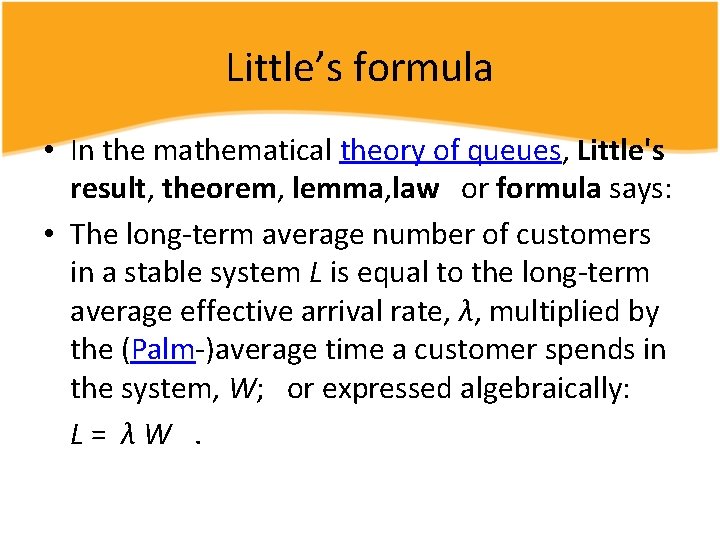
Little’s formula • In the mathematical theory of queues, Little's result, theorem, lemma, law or formula says: • The long-term average number of customers in a stable system L is equal to the long-term average effective arrival rate, λ, multiplied by the (Palm-)average time a customer spends in the system, W; or expressed algebraically: L = λ W.

Little’s formula • The only requirements are that the system is stable and non-preemptive; this rules out transition states such as initial startup or shutdown. • In some cases it is possible to mathematically relate not only the average number in the system to the average wait but relate the entire probability distribution (and moments) of the number in the system to the wait.

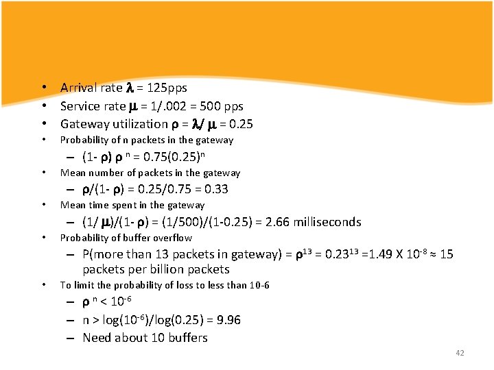
M/M/1 Example • On a network gateway, measurements show that the packets arrive at a mean rate of 125 packets per seconds(pps) and the gateway takes about two milliseconds to forward them. Using an M/M/1 model, analyze the gateway. What is the probability of buffer overflow if the gateway had only 13 buffers? How many buffers do we need to keep packet loss below one packet per million? 41

• Arrival rate = 125 pps • Service rate = 1/. 002 = 500 pps • Gateway utilization ρ = / = 0. 25 • Probability of n packets in the gateway – (1 - ρ) ρ n = 0. 75(0. 25)n • Mean number of packets in the gateway – ρ/(1 - ρ) = 0. 25/0. 75 = 0. 33 • Mean time spent in the gateway – (1/ )/(1 - ρ) = (1/500)/(1 -0. 25) = 2. 66 milliseconds • Probability of buffer overflow – P(more than 13 packets in gateway) = ρ13 = 0. 2313 =1. 49 X 10 -8 ≈ 15 packets per billion packets • To limit the probability of loss to less than 10 -6 – ρ n < 10 -6 – n > log(10 -6)/log(0. 25) = 9. 96 – Need about 10 buffers 42

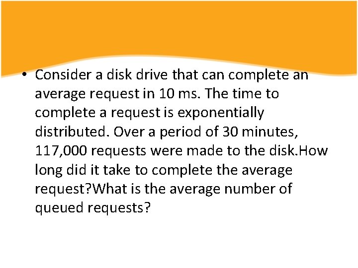
• Consider a disk drive that can complete an average request in 10 ms. The time to complete a request is exponentially distributed. Over a period of 30 minutes, 117, 000 requests were made to the disk. How long did it take to complete the average request? What is the average number of queued requests?

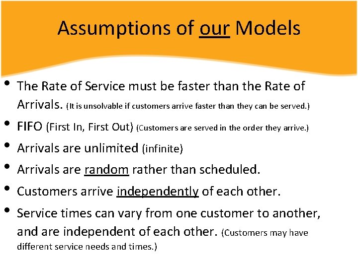
Assumptions of our Models • The Rate of Service must be faster than the Rate of Arrivals. (It is unsolvable if customers arrive faster than they can be served. ) • FIFO (First In, First Out) (Customers are served in the order they arrive. ) • Arrivals are unlimited (infinite) • Arrivals are random rather than scheduled. • Customers arrive independently of each other. • Service times can vary from one customer to another, and are independent of each other. (Customers may have different service needs and times. )