Process simulation optimisation and design P S O

Process simulation, optimisation and design

P. S. O. D. ORGANIZATION ISSUES

Course scope Introduction n Math. CAD n Introduction to CAPE n Simple simulation of heat exchange process using common software n Chem. CAD (by dr Robert Kubica) n

Process simulation, optimisation and design Course objectives

n Provide the students with: – using specialized software for mathematical problems solution – clear understanding of what is a process simulation, a process optimization and process design – using commonly available software to solve simulation problems – using specialized software for process simulation

Lectures are available on the web address www. chemia. polsl. pl/~jkocurek/Studenci. html

Introduction

All the simulation related issues requires

A Model, what is it? n A model is a representation of some aspects of real world objects by: – other parameters easier to measure – scaled down objects – equations and numbers – mathematical models

The Model, what for? n A good model of the apparatus is needed for: – Apparatus design – Process » simulation » optimization » design n apparatus design can be done with pen and piece of paper but even quite simple process optimization problem needs to involve the computer

Model, how to calculate? n Manually – We need: » Knowledge » Paper and pen » Log tables, slide rule, calculator n Computer supported calculation – We need: » Knowledge » PROGRAM

COMPUTER PROGRAM DEFINITION „Set of instructions in a logical sequence interpreted and executed by a computer enabling the computer to perform a required function; also called software. Programs are the "thought processes" of computers, without which they cannot operate. Programs are written in various languages, to conform with the operating system of particular computers. ”

Computer supported calculation n PROGRAM – Written by user, using programming language: » Low level (assembler) » High level (C, Pascal, Fortran, Basic) – Written by user, using common applications for calculation » Spreadsheets (Excel, Calc) » Mathematical tools (Math. Lab, Math. CAD) – Specialized software for modeling and process simulation (Aspen. One, Pro. SIM, Chem. CAD)

Math. CAD The mathematical tool

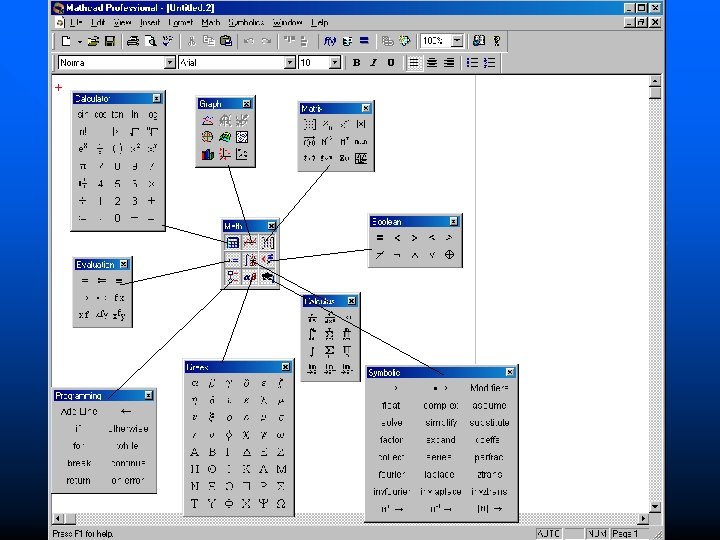
Introduction n User interface – Writing cursor '+' – Toolbars » » » » » Calculator – equation symbols Graph – building the charts Matrix – inserting matrix/vectors, matrics operation Calculus – derivatives, integrals, limits, summation, iterated product Symbolic Evaluation Boolean –logical operation Programming Greek – inserting Greek letters – Turn of the Resource center at startup View/Preferences/Startup Options

n Basic operations – Typing: » "normal" – text n n Forced by: [shift]+["] Automatically: after space insertion » "variable" – interpreted by program n Default – The typing modes are identified by style: » Normal – Font is Arial (by default) » Variable – Font is Times (by default) – Assign symbol": =" (keys [: ][=])

n Numbers notation – Floating-point notation: 1. 23· 104 Multiplication symbol [*] Superscript (exponent) [^] Key sequence: [1][. ][2][3][*][1][0][^][4]

Math. CAD intro n Algebraic expressions – +, -, / +, -, , *(not always needed), power [^] – Functions arguments "(. . . )" – Result (evaluation): [=] n Expression typing – standard mathematical notation: [2][/][3][+][3][^][2][ ][l][n][(][3][)][=] or [2][/][3][+][3][^][2][space bar][l][n][(][3][)][=] To go back to basic level press spacebar or right arrow

Math. CAD intro n Variables notation – Latin and Greek alphabet ( [ctrl] + [g] after typing Latin letter) – Case sensitivity: x X – Subscripts (not vector/matrix subscripts) [. ] – Prim: x`, bis: x`` etc.

Math. CAD intro n Assigning values and expressions (Pascal like) – One value assigned to one variable: x: =5 keys: [x][: ][5] – Range of arithmetic progression assigned to variable » Default step: x: =0. . 3 (means numbers 0, 1, 2, 3) keys [x][: ][0][; ][3] » Defined step: x: =0, 2. . 6 (means numbers 0, 2, 4, 6) keys [x][: ][0][, ][2][; ][6] Has to be defined earlier – Expression to variable: y: =2·x+3 keys: [y][: ][2][*][x][+][3]

Math. CAD intro Correct Incorrect

Math. CAD intro n The expressions edition – To change the position of edited place press space bar Vertical line: shows place of insertion of a sign Horizontal: shows range will be inserted into function etc.

Math. CAD functions n n Standard functions set Functions definition – Syntax: Function. Name(arg 1, arg 2, . . . ): = expression – E. g. f(x, y)=x·y keys: [f][(][x][y][)][: ][x][*][y] n Calculations with use of defined (or predefined) functions: – – – Evaluation for constants Evaluation for defined variables Evaluation for range of constants (vectors)

Math. CAD functions n Function of constant (scalar)

Math. CAD functions n Function of variable Global variable Local variable

Math. CAD functions n Range of arithmetic sequence (or vector)

Math. CAD functions n Graphs: – Function of one variable f(x) keys: [f][(][x][)][shift]+[2][x]

Math. CAD functions n Graphs: – Default independent values range: -10 ÷ 10 – Can be edited

Math. CAD functions n Graphs: – Several functions of one independent variable range: f(x), g(x)@x keys: [f][(][x][)][, ] [g][(][x][)][shift]+[2][x]

Math. CAD functions n Graphs: – Several functions of several different independent variable range: f(x), g(z)@x, z keys: [f][(][x][)][, ] [g][(][z][)][shift]+[2][x][, ][z]

Math. CAD functions n Graphs formatting:

Math. CAD functions n Graphs formatting:

Math. CAD functions

Math. CAD functions Show markers enabled

Math. CAD – vectors and matrix Matrix variable definition n vector – one column matrix n

Math. CAD – vectors and matrix

Math. CAD – vectors and matrix n Matrix operations – – – Multiply by constant Matrix transpose [ctrl]+[1] Inverse [^][-][1] Matrix multiplying Determinant

Math. CAD – vectors and matrix n To read the matrix elements Ar, k: key [[] rrow nr, k – column nr – e. g. element A 1, 1 keys: [A][[][1][, ][1][=] n To chose matrix column – First column A( A<0>): keys [A][ctrl]+[6][0] – Default first column number is 0, (to change : Math/Options/Array Origin)

Math. CAD – vectors and matrix n Calculations of dot product and cross product of vectors

Math. CAD – vectors and matrix n Special definition of matrix elements as a function of row-column number Mi, j=f(i, j) – E. g. Value of element is equal to product of column and row number

n Math. CAD 3 D graphs of function on the base of matrix : [ctrl]+[2][M] – M – matrix defined earlier RESTICTION: function arguments have to bee integer type

Math. CAD 3 D graphs n 3 D Graphs of function of real type arguments – Using procedure: Create. Mesh(function, lb_v 1, ub_v 1, lb_v 2, ub_v 2, v 1 grid, v 2 grid) – Assign result to variable – Plot of the variable like plot of matrix ([ctrl]+[2]) Boundaries can be the real type numbers. (def. – 5, 5) Grids have to be integer type numbers (def. 20)

Math. CAD 3 D graphs

Math. CAD 3 D graphs - formating

Math. CAD 3 D graphs – formatting: fill options

Math. CAD 3 D graphs – formatting: fill options Contours colour filled

Math. CAD 3 D graphs – formatting: line options

Math. CAD 3 D graphs – formatting: Lighting

Math. CAD 3 D graphs – formatting: Fog and perspective

Math. CAD 3 D graphs – formatting: Backplane and Grids

Predefined constants n n n e = 2, 718 – natural logarithm base g = 9, 81 m 2/s – acceleration of gravity = 3, 142 – circle perimeter/diameter ratio

Math. CAD equation solving n Single equation (one unknown value) 1. Given-Find method » » Input start point of variable Type "Given" Type equation with using [=] ([ctrl]+[=]) Type Find(variable)=

Math. CAD equation solving n Given-Find – solving methods – – Linear (function of type c 0 x 0 + c 1 x 1 +. . . + cnxn) – starting point do not affects on results, it only defines size of matrix/vector of the solution. Nonlinear – according to nonlinear equation. Obtained result could depend on starting point. Available methods: » » n Conjugate Gradient Quasi – Newton Levenberg-Marquardt Quadratic The choice of method is automatic by default. User can choose method from the pop-up menu over word Find.

Math. CAD equation solving n Single equation (one unknown value) 2. Root procedure: Root(function, variable, low_limit, up_limit)= – Values of function at the bounds must have different signs or

Math. CAD equation solving n Single equation (one unknown value) 2. Root procedure methods: 1. Secant method 2. Mueller method y 1 x 2 y 3 y 2 x 3 x 5 x 4 x 1

n Math. CAD equation solving Single equation (one unknown value) 3. Special procedure: polyroots for the polynomials. Argument of procedure is a vector of polynomial coefficients (a 0, a 1. . . ). The result is a vector too. Methods: 1. Laguerre's method 2. companion matrix 3.

Math. CAD, the system of equations solving n The system of linear equations – Solving on the base of matrix toolbar: » Prepare square matrix of equations coefficients (A) and vector of free terms (B) » Do the operation x: =A-1 B and show result: x= Or » Use the procedure LSOLVE: lsolve(A, B)=

Math. CAD, the system of equations solving

Math. CAD, the system of equations solving n The system of nonlinear equation – Can be solved using given-find method » Assign starting values to variables » Type Given » Type the equations using = sign (bolded) » Type Find(var 1, var 2, . . . )=

Math. CAD, the system of equations solving

Differential equations solving n Numerical methods: – Gives only values not function – Engineer usually needs values – There is no need to make complicated transformations (e. g. variables separation) – Basic method implemented in Math. CAD is Runge-Kutta 4 th order method.

Differential equations solving n Numerical methods principle – Calculation involve bounded segment of independent variable only – Every point is being calculated on the base of one or few points calculated before or given. – Independent variable is calculated using step: x i+1 = x i + h = x i+ D x – Dependent value is being calculated according to the method

Differential equations solving n Runge-Kutta 4 th order method principles: – New point of integral is being calculated on the base of one point (given/calculated) and 4 intermediate values

Math. CAD differential equations n Single, first order differential equation Initial condition 1. Assign the initial value of dependent variable (optionally) 2. Define the derivative function 3. Assign to the new variable the integrating function rkfixed: R: =rkfixed(init_v, low_bound, up_bound, num_seg, function)

Math. CAD differential equations 4. Result is matrix (table) of two columns: first contain independent values second dependent ones 5. To show result as a plot: R<1>@R<0>

Math. CAD differential equations

Math. CAD differential equations n System of first order differential equations 1. Assign the vector of initial conditions of dependent variables (starting vector) 2. Define the vectoral function of derivatives (right-hand sides of equations) 3. Assign to the variable function rkfixed: R: =rkfixed(init_vect, low_bound, up_bound, num_seg, function)

Math. CAD differential equations 4. Result is matrix (table) of three columns: first contain independent values, 2 nd first dependent values, third second ones : 5. Results as a plot: R<1>, R<2>@ R<0>

Math. CAD differential equations

n Math. CAD differential equations Single second order equation Initial condition 1. Transform the second order equation to the system of two first order equations:

Math. CAD differential equations Example: Solve the second order differential equation (calculate values of function and its first derivatives) given by equation: n While y=10 and y’=-1 for x=0 In the range of x=<0, 1>

Math. CAD differential equations System of equations Starting vector Vectoral function