Prerequisites Almost essential Firm Optimisation Consumption Basics Frank

Prerequisites Almost essential Firm: Optimisation Consumption: Basics Frank Cowell: Microeconomics October 2006 Consumer Optimisation MICROECONOMICS Principles and Analysis Frank Cowell

What we're going to do: Frank Cowell: Microeconomics Jump to “Firm” n n We’ll solve the consumer's optimisation problem. . . using methods that we've already introduced. This enables us to re-cycle old techniques and results. A tip: u u u Run the presentation for firm optimisation… look for the points of comparison. . . and try to find as many reinterpretations as possible.

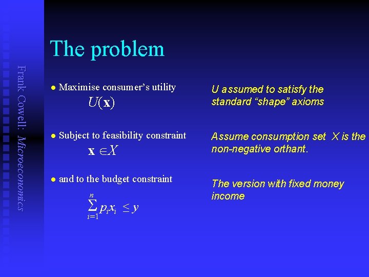
The problem Frank Cowell: Microeconomics n Maximise consumer’s utility U(x) U assumed to satisfy the standard “shape” axioms n Subject to feasibility constraint Assume consumption set X is the non-negative orthant. n and to the budget constraint The version with fixed money income x X n S pixi i=1 ≤y

Overview. . . Frank Cowell: Microeconomics Two fundamental views of consumer optimisation Consumer: Optimisation Primal and Dual problems Lessons from the Firm Primal and Dual again

An obvious approach? Frank Cowell: Microeconomics n We now have the elements of a standard constrained optimisation problem: u u n The next steps might seem obvious: u u u n n the constraints on the consumer. the objective function. set up a standard Lagrangean. solve it. interpret the solution. But the obvious approach is not always the most insightful. We’re going to try something a little sneakier…

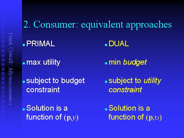
Think laterally. . . Frank Cowell: Microeconomics n n n In microeconomics an optimisation problem can often be represented in more than one form. Which form you use depends on the information you want to get from the solution. This applies here. The same consumer optimisation problem can be seen in two different ways. I’ve used the labels “primal” and “dual” that have become standard in the literature.

A five-point plan Frank Cowell: Microeconomics The primal problem n n n Set out the basic consumer optimisation problem. The dual problem Show that the solution is equivalent to another problem. Show that this equivalent problem is identical to that of the firm. The primal problem again Write down the solution. Go back to the problem we first thought of. . .

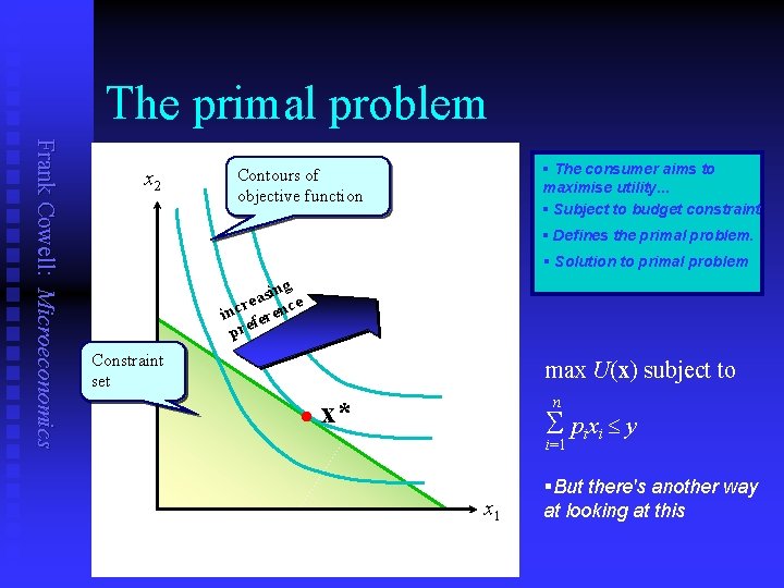
The primal problem Frank Cowell: Microeconomics x 2 § The consumer aims to maximise utility. . . § Subject to budget constraint Contours of objective function § Defines the primal problem. § Solution to primal problem ing s a e re inc ferenc pre Constraint set max U(x) subject to l n x* S pixi y i=1 x 1 §But there's another way at looking at this

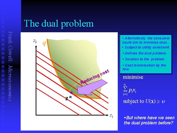
The dual problem Frank Cowell: Microeconomics xz 2 uq § Alternatively the consumer could aim to minimise cost. . . § Subject to utility constraint Constraint set § Defines the dual problem. § Solution to the problem l l ost c ng i c du ost c Re ng i c du e R x* z* Contours of objective function § Cost minimisation by the firm minimise n S pixi i=1 subject to U(x) u xz 1 §But where have we seen the dual problem before?

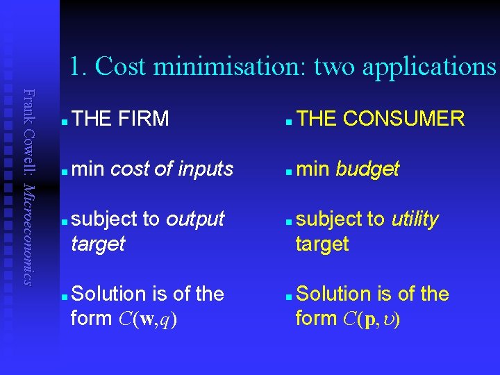
Two types of cost minimisation Frank Cowell: Microeconomics n n The similarity between the two problems is not just a curiosity. We can use it to save ourselves work. All the results that we had for the firm's “stage 1” problem can be used. We just need to “translate” them intelligently u Swap over the symbols u Swap over the terminology u Relabel theorems

Overview. . . Frank Cowell: Microeconomics Reusing results on optimisation Consumer: Optimisation Primal and Dual problems Lessons from the Firm Primal and Dual again

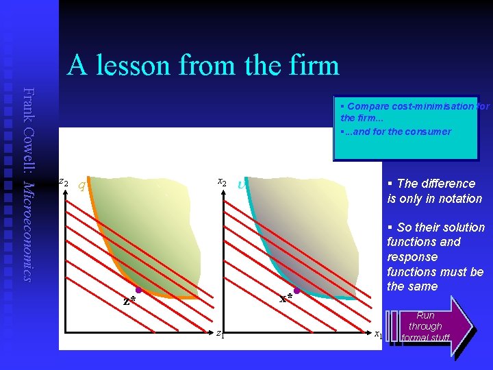
A lesson from the firm Frank Cowell: Microeconomics § Compare cost-minimisation for the firm. . . §. . . and for the consumer z 2 x 2 q l u § The difference is only in notation § So their solution functions and response functions must be the same l x* z* z 1 x 1 Run through formal stuff

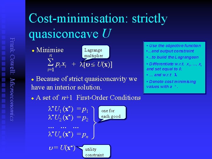
Frank Cowell: Microeconomics Cost-minimisation: strictly quasiconcave U l Minimise Lagrange multiplier n S pi xi i=1 + l[u U(x)] u – U(x) Because of strict quasiconcavity we have an interior solution. l A set of n+1 First-Order Conditions l l* U 1 (x* ) = p 1 l* U 2 (x* ) = p 2 … … … l* Un (x* ) = pn u = U(x* ) ü ý þ one for each good utility constraint § Use the objective function §. . . and output constraint §. . . to build the Lagrangean § Differentiate w. r. t. x 1, . . . , xn and set equal to 0. §. . . and w. r. t l § Denote cost minimising values with a *.

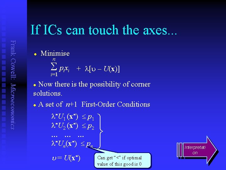
If ICs can touch the axes. . . Frank Cowell: Microeconomics l Minimise n S pixi i=1 + l[u – U(x)] Now there is the possibility of corner solutions. l A set of n+1 First-Order Conditions l l*U 1 (x*) p 1 l*U 2 (x*) p 2 … … … l*Un(x*) pn u = U(x*) ü ý þ Can get “<” if optimal value of this good is 0 Interpretati on

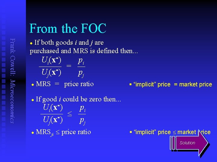
From the FOC Frank Cowell: Microeconomics If both goods i and j are purchased and MRS is defined then. . . l Ui(x*) pi ——— = — * Uj(x ) pj l MRS = price ratio l If good i could be zero then. . . l MRSji price ratio § “implicit” price = market price Ui(x*) pi ——— — * Uj(x ) pj § “implicit” price market price Solution

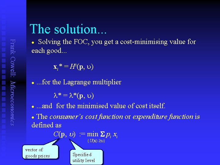
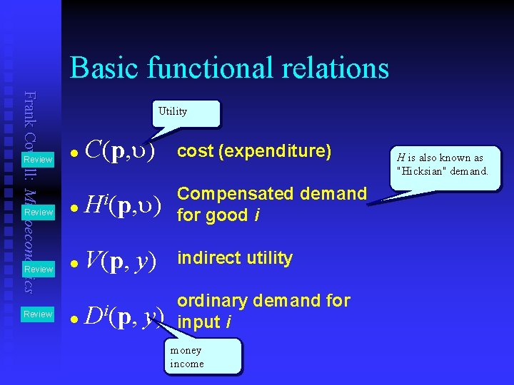
The solution. . . Frank Cowell: Microeconomics Solving the FOC, you get a cost-minimising value for each good. . . l xi* = Hi(p, u) l . . . for the Lagrange multiplier l* = l*(p, u) l. . . and for the minimised value of cost itself. l The consumer’s cost function or expenditure function is defined as C(p, u) : = min S pi xi {U(x) u} vector of goods prices Specified utility level

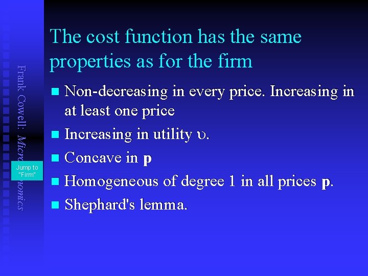
Frank Cowell: Microeconomics Jump to “Firm” The cost function has the same properties as for the firm Non-decreasing in every price. Increasing in at least one price n Increasing in utility u. n Concave in p n Homogeneous of degree 1 in all prices p. n Shephard's lemma. n

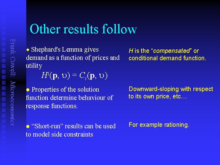
Other results follow Frank Cowell: Microeconomics Shephard's Lemma gives demand as a function of prices and utility H is the “compensated” or conditional demand function. Properties of the solution function determine behaviour of response functions. Downward-sloping with respect to its own price, etc… “Short-run” results can be used to model side constraints For example rationing. n Hi(p, u) = Ci(p, u) n n

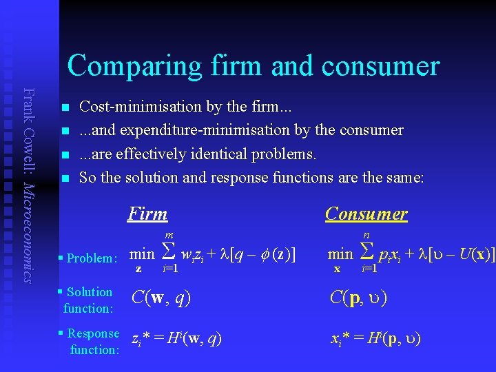
Comparing firm and consumer Frank Cowell: Microeconomics n n Cost-minimisation by the firm. . . and expenditure-minimisation by the consumer. . . are effectively identical problems. So the solution and response functions are the same: Firm Consumer m § Problem: min z § Solution function: S wizi + l[q – f (z)] i=1 C(w, q) § Response z * = Hi(w, q) function: i n min x S pixi + l[u – U(x)] i=1 C(p, u) xi* = Hi(p, u)

Overview. . . Frank Cowell: Microeconomics Exploiting the two approaches Consumer: Optimisation Primal and Dual problems Lessons from the Firm Primal and Dual again

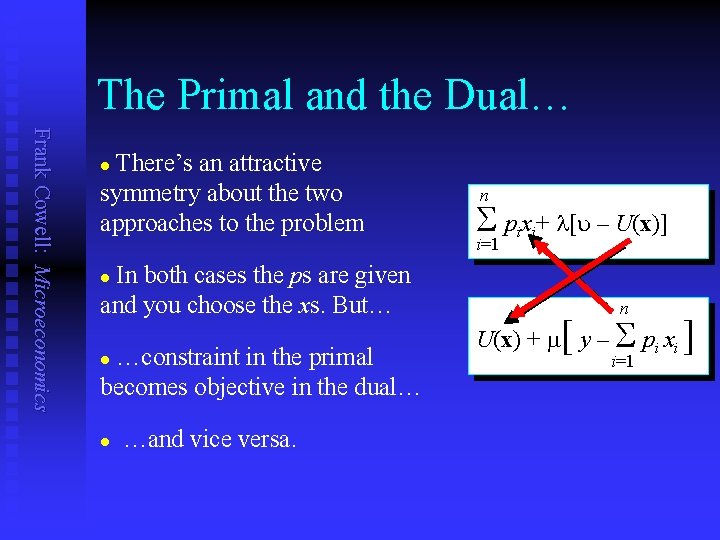
The Primal and the Dual… Frank Cowell: Microeconomics There’s an attractive symmetry about the two approaches to the problem l In both cases the ps are given and you choose the xs. But… n S pixi+ l[u – U(x)] i=1 l …constraint in the primal becomes objective in the dual… l l …and vice versa. n U(x) + m y – S pi xi [ i=1 ]

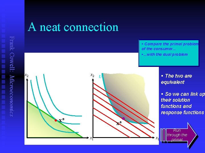
A neat connection Frank Cowell: Microeconomics § Compare the primal problem of the consumer. . . §. . . with the dual problem x 2 u § The two are equivalent § So we can link up their solution functions and response functions l l x* x* x 1 Run through the primal

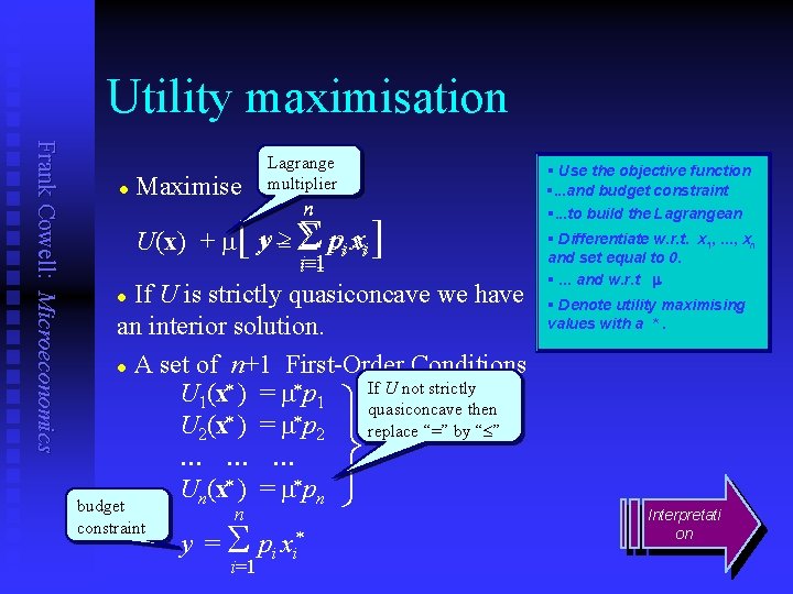
Utility maximisation Frank Cowell: Microeconomics l Maximise Lagrange multiplier n U(x) + m y – S ppii xxii [ i=1 ] If U is strictly quasiconcave we have an interior solution. l A set of n+1 First-Order Conditions If U not strictly U 1(x* ) = m* p 1 one for quasiconcave then each good U 2(x* ) = m* p 2 replace “=” by “ ” … … … Un(x* ) = m* pn l budget constraint n y = S pi xi* i=1 ü ý þ § Use the objective function §. . . and budget constraint §. . . to build the Lagrangean § Differentiate w. r. t. x 1, . . . , xn and set equal to 0. §. . . and w. r. t m § Denote utility maximising values with a *. Interpretati on

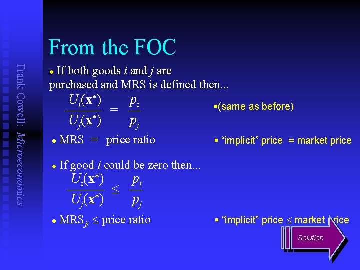
From the FOC Frank Cowell: Microeconomics If both goods i and j are purchased and MRS is defined then. . . l Ui(x*) pi ——— = — * Uj(x ) pj l MRS = price ratio l If good i could be zero then. . . l MRSji price ratio §(same as before) § “implicit” price = market price Ui(x*) pi ——— — * Uj(x ) pj § “implicit” price market price Solution

The solution. . . Frank Cowell: Microeconomics Solving the FOC, you get a utility-maximising value for each good. . . xi* = Di(p, y) l l . . . for the Lagrange multiplier m* = m*(p, y) . . . and for the maximised value of utility itself. l The indirect utility function is defined as l V(p, y) : = max U(x) {S pixi y} vector of goods prices money income

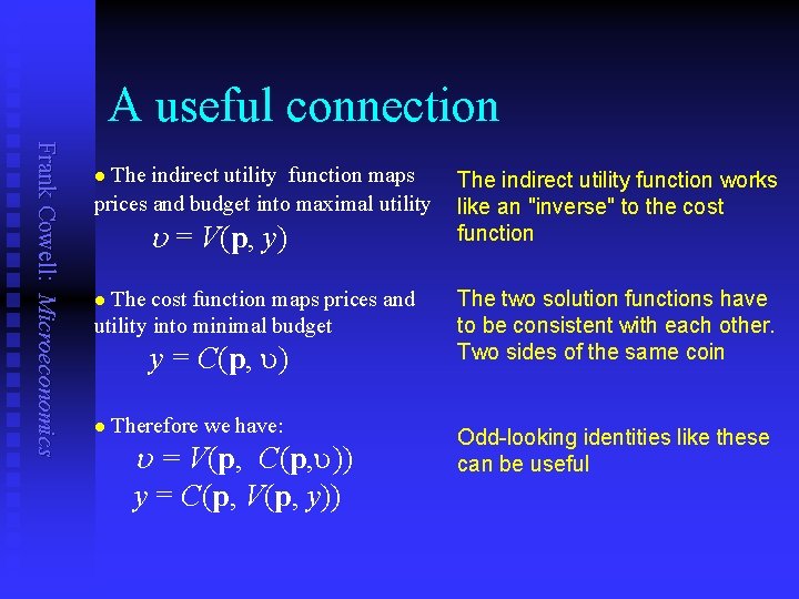
A useful connection Frank Cowell: Microeconomics The indirect utility function maps prices and budget into maximal utility The indirect utility function works like an "inverse" to the cost function The cost function maps prices and utility into minimal budget The two solution functions have to be consistent with each other. Two sides of the same coin n u = V(p, y) n y = C(p, u) n Therefore we have: u = V(p, C(p, u)) y = C(p, V(p, y)) Odd-looking identities like these can be useful

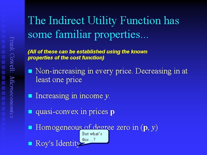
Frank Cowell: Microeconomics The Indirect Utility Function has some familiar properties. . . (All of these can be established using the known properties of the cost function) n Non-increasing in every price. Decreasing in at least one price n Increasing in income y. n quasi-convex in prices p n Homogeneous of degree zero in (p, y) n Roy's Identity But what’s this…?

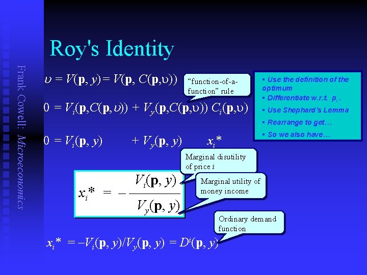
Roy's Identity Frank Cowell: Microeconomics u = V(p, y)= V(p, C(p, u)) “function-of-afunction” rule 0 = Vi(p, C(p, u)) + Vy(p, C(p, u)) Ci(p, u) § Use the definition of the optimum § Differentiate w. r. t. pi. § Use Shephard’s Lemma § Rearrange to get… 0 = Vi(p, y) + Vy(p, y) x i* § So we also have… Marginal disutility of price i Vi(p, y) xi* = – ———— Vy(p, y) Marginal utility of money income Ordinary demand function xi* = –Vi(p, y)/Vy(p, y) = Di(p, y)

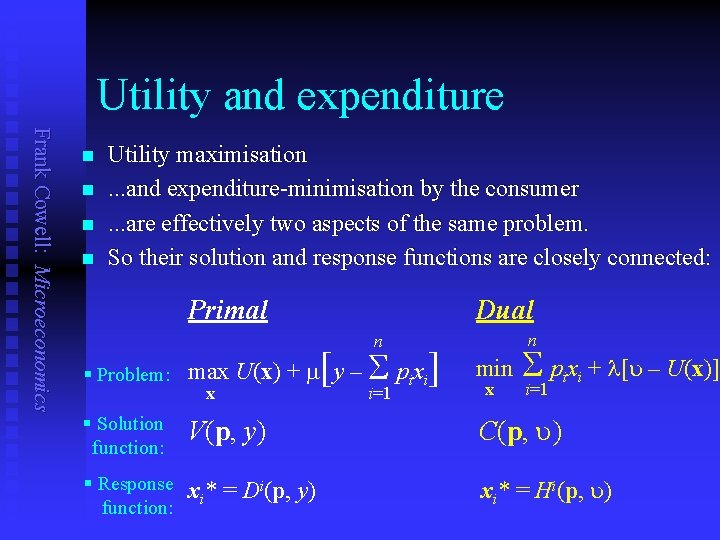
Utility and expenditure Frank Cowell: Microeconomics n n Utility maximisation. . . and expenditure-minimisation by the consumer. . . are effectively two aspects of the same problem. So their solution and response functions are closely connected: Primal Dual n n [ S px] § Problem: max U(x) + m y – x § Solution function: V(p, y) § Response x * = Di(p, y) function: i i=1 i i min x S pixi + l[u – U(x)] i=1 C(p, u) xi* = Hi(p, u)

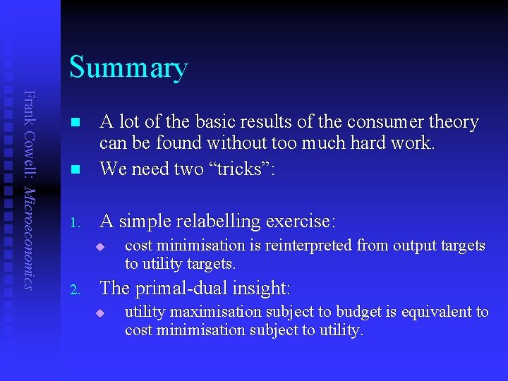
Summary Frank Cowell: Microeconomics n A lot of the basic results of the consumer theory can be found without too much hard work. We need two “tricks”: 1. A simple relabelling exercise: n u 2. cost minimisation is reinterpreted from output targets to utility targets. The primal-dual insight: u utility maximisation subject to budget is equivalent to cost minimisation subject to utility.

1. Cost minimisation: two applications Frank Cowell: Microeconomics n THE FIRM n THE CONSUMER n min cost of inputs n min budget n n subject to output target Solution is of the form C(w, q) n n subject to utility target Solution is of the form C(p, u)

2. Consumer: equivalent approaches Frank Cowell: Microeconomics n PRIMAL n DUAL n max utility n min budget n n subject to budget constraint Solution is a function of (p, y) n n subject to utility constraint Solution is a function of (p, u)

Basic functional relations Frank Cowell: Microeconomics Utility l C(p, u) Review l Compensated demand i H (p, u) Review l V(p, y) indirect utility l Di(p, ordinary demand for input i Review cost (expenditure) for good i y) money income H is also known as "Hicksian" demand.

What next? Frank Cowell: Microeconomics Examine the response of consumer demand to changes in prices and incomes. n Household supply of goods to the market. n Develop the concept of consumer welfare n