PART A Ordinary Differential Equations ODEs Section 1

PART A Ordinary Differential Equations (ODEs) Section 1. 1 p 1 Advanced Engineering Mathematics, 10/e by Edwin Kreyszig Copyright 2011 by John Wiley & Sons. All rights reserved.

1 CHAPTER First-Order ODEs Section 1. 1 p 2 Advanced Engineering Mathematics, 10/e by Edwin Kreyszig Copyright 2011 by John Wiley & Sons. All rights reserved.

1. 1 Section 1. 1 p 3 Basic Concepts. Modeling Advanced Engineering Mathematics, 10/e by Edwin Kreyszig Copyright 2011 by John Wiley & Sons. All rights reserved.

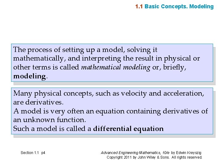
1. 1 Basic Concepts. Modeling The process of setting up a model, solving it mathematically, and interpreting the result in physical or other terms is called mathematical modeling or, briefly, modeling. Many physical concepts, such as velocity and acceleration, are derivatives. A model is very often an equation containing derivatives of an unknown function. Such a model is called a differential equation Section 1. 1 p 4 Advanced Engineering Mathematics, 10/e by Edwin Kreyszig Copyright 2011 by John Wiley & Sons. All rights reserved.

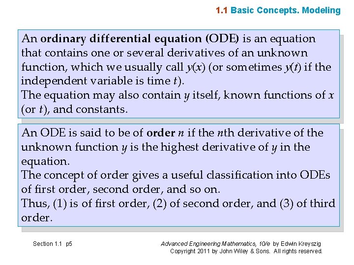
1. 1 Basic Concepts. Modeling An ordinary differential equation (ODE) is an equation that contains one or several derivatives of an unknown function, which we usually call y(x) (or sometimes y(t) if the independent variable is time t). The equation may also contain y itself, known functions of x (or t), and constants. An ODE is said to be of order n if the nth derivative of the unknown function y is the highest derivative of y in the equation. The concept of order gives a useful classification into ODEs of first order, second order, and so on. Thus, (1) is of first order, (2) of second order, and (3) of third order. Section 1. 1 p 5 Advanced Engineering Mathematics, 10/e by Edwin Kreyszig Copyright 2011 by John Wiley & Sons. All rights reserved.

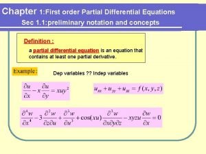
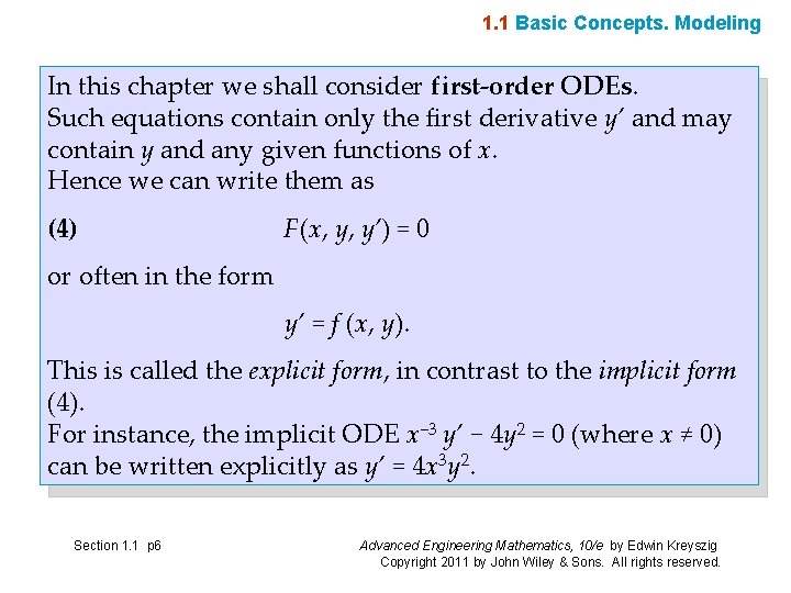
1. 1 Basic Concepts. Modeling In this chapter we shall consider first-order ODEs. Such equations contain only the first derivative y’ and may contain y and any given functions of x. Hence we can write them as (4) F(x, y, y’) = 0 or often in the form y’ = f (x, y). This is called the explicit form, in contrast to the implicit form (4). For instance, the implicit ODE x− 3 y’ − 4 y 2 = 0 (where x ≠ 0) can be written explicitly as y’ = 4 x 3 y 2. Section 1. 1 p 6 Advanced Engineering Mathematics, 10/e by Edwin Kreyszig Copyright 2011 by John Wiley & Sons. All rights reserved.

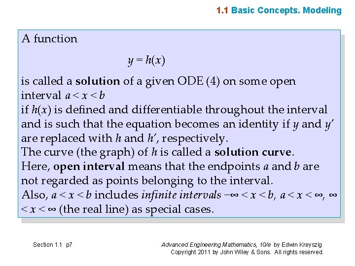
1. 1 Basic Concepts. Modeling A function y = h(x) is called a solution of a given ODE (4) on some open interval a < x < b if h(x) is defined and differentiable throughout the interval and is such that the equation becomes an identity if y and y’ are replaced with h and h’, respectively. The curve (the graph) of h is called a solution curve. Here, open interval means that the endpoints a and b are not regarded as points belonging to the interval. Also, a < x < b includes infinite intervals −∞ < x < b, a < x < ∞, ∞ < x < ∞ (the real line) as special cases. Section 1. 1 p 7 Advanced Engineering Mathematics, 10/e by Edwin Kreyszig Copyright 2011 by John Wiley & Sons. All rights reserved.

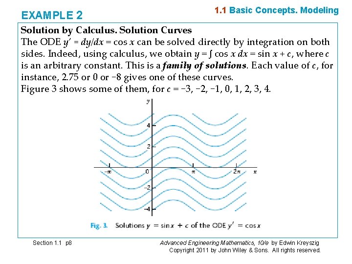
EXAMPLE 2 1. 1 Basic Concepts. Modeling Solution by Calculus. Solution Curves The ODE y’ = dy/dx = cos x can be solved directly by integration on both sides. Indeed, using calculus, we obtain y = ∫ cos x dx = sin x + c, where c is an arbitrary constant. This is a family of solutions. Each value of c, for instance, 2. 75 or 0 or − 8 gives one of these curves. Figure 3 shows some of them, for c = − 3, − 2, − 1, 0, 1, 2, 3, 4. Section 1. 1 p 8 Advanced Engineering Mathematics, 10/e by Edwin Kreyszig Copyright 2011 by John Wiley & Sons. All rights reserved.

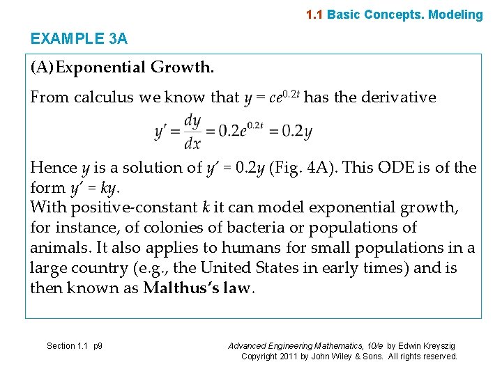
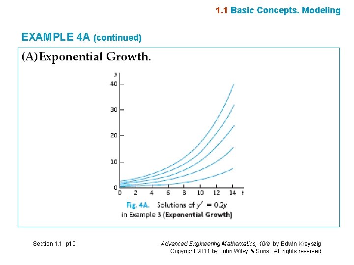
1. 1 Basic Concepts. Modeling EXAMPLE 3 A (A)Exponential Growth. From calculus we know that y = ce 0. 2 t has the derivative Hence y is a solution of y’ = 0. 2 y (Fig. 4 A). This ODE is of the form y’ = ky. With positive-constant k it can model exponential growth, for instance, of colonies of bacteria or populations of animals. It also applies to humans for small populations in a large country (e. g. , the United States in early times) and is then known as Malthus’s law. Section 1. 1 p 9 Advanced Engineering Mathematics, 10/e by Edwin Kreyszig Copyright 2011 by John Wiley & Sons. All rights reserved.

1. 1 Basic Concepts. Modeling EXAMPLE 4 A (continued) (A)Exponential Growth. Section 1. 1 p 10 Advanced Engineering Mathematics, 10/e by Edwin Kreyszig Copyright 2011 by John Wiley & Sons. All rights reserved.

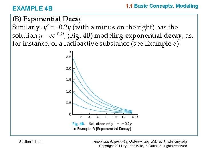
EXAMPLE 4 B 1. 1 Basic Concepts. Modeling (B) Exponential Decay Similarly, y’ = − 0. 2 y (with a minus on the right) has the solution y = ce− 0. 2 t, (Fig. 4 B) modeling exponential decay, as, for instance, of a radioactive substance (see Example 5). Section 1. 1 p 11 Advanced Engineering Mathematics, 10/e by Edwin Kreyszig Copyright 2011 by John Wiley & Sons. All rights reserved.

1. 1 Basic Concepts. Modeling We see that each ODE in these examples has a solution that contains an arbitrary constant c. Such a solution containing an arbitrary constant c is called a general solution of the ODE. (We shall see that c is sometimes not completely arbitrary but must be restricted to some interval to avoid complex expressions in the solution. ) We shall develop methods that will give general solutions uniquely (perhaps except for notation). Hence we shall say the general solution of a given ODE (instead of a general solution). Section 1. 1 p 12 Advanced Engineering Mathematics, 10/e by Edwin Kreyszig Copyright 2011 by John Wiley & Sons. All rights reserved.

1. 1 Basic Concepts. Modeling Geometrically, the general solution of an ODE is a family of infinitely many solution curves, one for each value of the constant c. If we choose a specific c (e. g. , c = 6. 45 or 0 or − 2. 01) we obtain what is called a particular solution of the ODE. A particular solution does not contain any arbitrary constants. In most cases, general solutions exist, and every solution not containing an arbitrary constant is obtained as a particular solution by assigning a suitable value to c. Exceptions to these rules occur but are of minor interest in applications. Section 1. 1 p 13 Advanced Engineering Mathematics, 10/e by Edwin Kreyszig Copyright 2011 by John Wiley & Sons. All rights reserved.

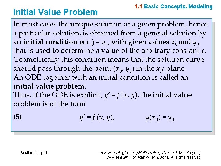
1. 1 Basic Concepts. Modeling Initial Value Problem In most cases the unique solution of a given problem, hence a particular solution, is obtained from a general solution by an initial condition y(x 0) = y 0, with given values x 0 and y 0, that is used to determine a value of the arbitrary constant c. Geometrically this condition means that the solution curve should pass through the point (x 0, y 0) in the xy-plane. An ODE together with an initial condition is called an initial value problem. Thus, if the ODE is explicit, y’ = f (x, y), the initial value problem is of the form (5) Section 1. 1 p 14 y’ = f (x, y), y(x 0) = y 0. Advanced Engineering Mathematics, 10/e by Edwin Kreyszig Copyright 2011 by John Wiley & Sons. All rights reserved.

1. 1 Basic Concepts. Modeling EXAMPLE 5 Radioactivity. Exponential Decay Given an amount of a radioactive substance, say, 0. 5 g (gram), find the amount present at any later time. Physical Information. Experiments show that at each instant a radioactive substance decomposes—and is thus decaying in time—proportional to the amount of substance present. Section 1. 1 p 15 Advanced Engineering Mathematics, 10/e by Edwin Kreyszig Copyright 2011 by John Wiley & Sons. All rights reserved.

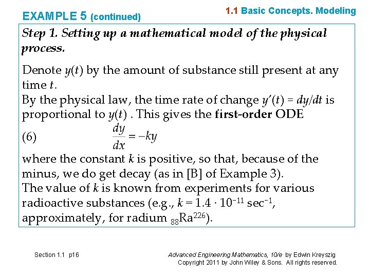
EXAMPLE 5 (continued) 1. 1 Basic Concepts. Modeling Step 1. Setting up a mathematical model of the physical process. Denote y(t) by the amount of substance still present at any time t. By the physical law, the time rate of change y’(t) = dy/dt is proportional to y(t). This gives the first-order ODE (6) where the constant k is positive, so that, because of the minus, we do get decay (as in [B] of Example 3). The value of k is known from experiments for various radioactive substances (e. g. , k = 1. 4 · 10− 11 sec− 1, approximately, for radium 88 Ra 226). Section 1. 1 p 16 Advanced Engineering Mathematics, 10/e by Edwin Kreyszig Copyright 2011 by John Wiley & Sons. All rights reserved.

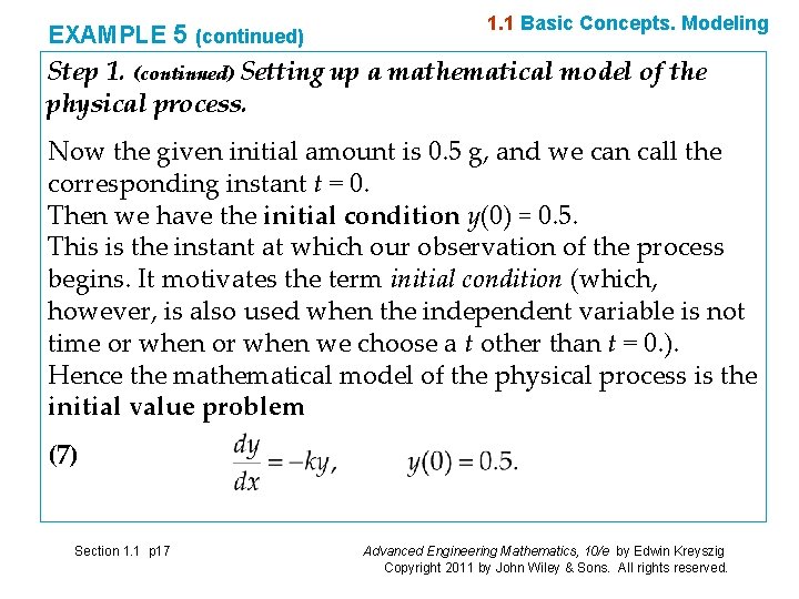
EXAMPLE 5 (continued) 1. 1 Basic Concepts. Modeling Step 1. (continued) Setting up a mathematical model of the physical process. Now the given initial amount is 0. 5 g, and we can call the corresponding instant t = 0. Then we have the initial condition y(0) = 0. 5. This is the instant at which our observation of the process begins. It motivates the term initial condition (which, however, is also used when the independent variable is not time or when we choose a t other than t = 0. ). Hence the mathematical model of the physical process is the initial value problem (7) Section 1. 1 p 17 Advanced Engineering Mathematics, 10/e by Edwin Kreyszig Copyright 2011 by John Wiley & Sons. All rights reserved.

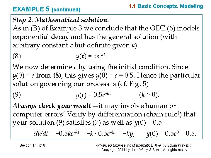
1. 1 Basic Concepts. Modeling EXAMPLE 5 (continued) Step 2. Mathematical solution. As in (B) of Example 3 we conclude that the ODE (6) models exponential decay and has the general solution (with arbitrary constant c but definite given k) (8) y(t) = ce−kt. We now determine c by using the initial condition. Since y(0) = c from (8), this gives y(0) = c = 0. 5. Hence the particular solution governing our process is (cf. Fig. 5) (9) y(t) = 0. 5 e−kt (k > 0). Always check your result—it may involve human or computer errors! Verify by differentiation (chain rule!) that your solution (9) satisfies (7) as well as y(0) = 0. 5: dy/dt = − 0. 5 ke−kt = −k · 0. 5 e−kt = −ky, Section 1. 1 p 18 y(0) = 0. 5 e 0 = 0. 5. Advanced Engineering Mathematics, 10/e by Edwin Kreyszig Copyright 2011 by John Wiley & Sons. All rights reserved.

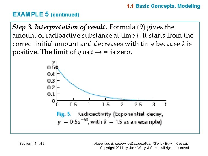
1. 1 Basic Concepts. Modeling EXAMPLE 5 (continued) Step 3. Interpretation of result. Formula (9) gives the amount of radioactive substance at time t. It starts from the correct initial amount and decreases with time because k is positive. The limit of y as t → ∞ is zero. Section 1. 1 p 19 Advanced Engineering Mathematics, 10/e by Edwin Kreyszig Copyright 2011 by John Wiley & Sons. All rights reserved.

1. 2 Geometric Meaning of y’ = f(x, y). Direction Fields, Euler’s Method Section 1. 2 p 20 Advanced Engineering Mathematics, 10/e by Edwin Kreyszig Copyright 2011 by John Wiley & Sons. All rights reserved.

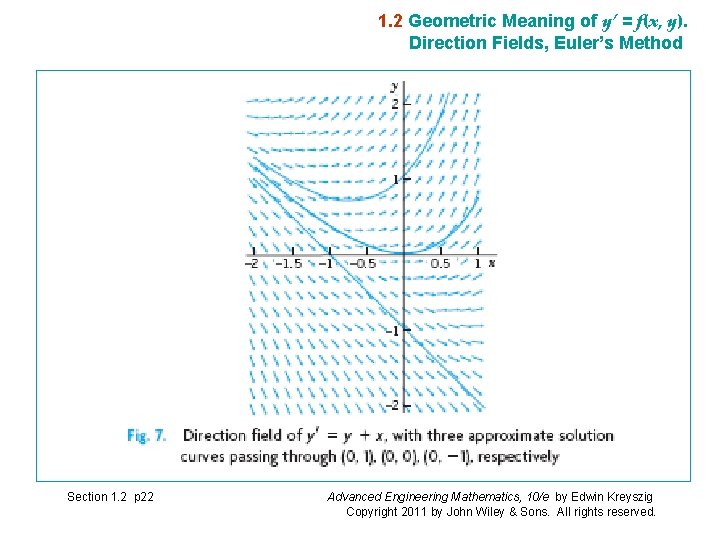
1. 2 Geometric Meaning of y’ = f(x, y). Direction Fields, Euler’s Method Graphic Method of Direction Fields. Practical Example Illustrated in Fig. 7. We can show directions of solution curves of a given ODE (1) by drawing short straight-line segments (lineal elements) in the xy-plane. This gives a direction field (or slope field) into which you can then fit (approximate) solution curves. This may reveal typical properties of the whole family of solutions. Figure 7 shows a direction field for the ODE (2) y’ = y + x obtained by a CAS (computer algebra system) and some approximate solution curves fitted in. Section 1. 2 p 21 Advanced Engineering Mathematics, 10/e by Edwin Kreyszig Copyright 2011 by John Wiley & Sons. All rights reserved.

1. 2 Geometric Meaning of y’ = f(x, y). Direction Fields, Euler’s Method Section 1. 2 p 22 Advanced Engineering Mathematics, 10/e by Edwin Kreyszig Copyright 2011 by John Wiley & Sons. All rights reserved.

1. 2 Geometric Meaning of y’ = f(x, y). Direction Fields, Euler’s Method If you have no CAS, first draw a few level curves f(x, y) = const of f(x, y), then parallel lineal elements along each such curve (which is also called an isocline, meaning a curve of equal inclination), and finally draw approximation curves fit to the lineal elements. Section 1. 2 p 23 Advanced Engineering Mathematics, 10/e by Edwin Kreyszig Copyright 2011 by John Wiley & Sons. All rights reserved.

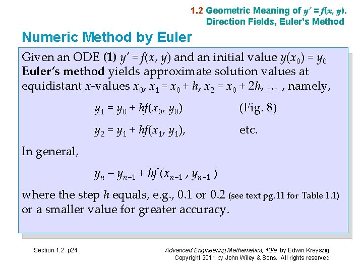
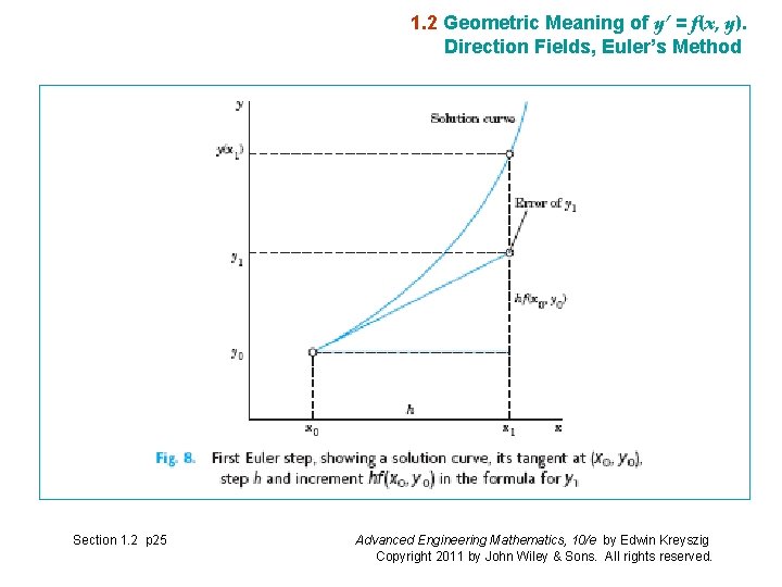
1. 2 Geometric Meaning of y’ = f(x, y). Direction Fields, Euler’s Method Numeric Method by Euler Given an ODE (1) y’ = f(x, y) and an initial value y(x 0) = y 0 Euler’s method yields approximate solution values at equidistant x-values x 0, x 1 = x 0 + h, x 2 = x 0 + 2 h, … , namely, y 1 = y 0 + hf(x 0, y 0) (Fig. 8) y 2 = y 1 + hf(x 1, y 1), etc. In general, yn = yn− 1 + hf (xn− 1 , yn− 1 ) where the step h equals, e. g. , 0. 1 or 0. 2 (see text pg. 11 for Table 1. 1) or a smaller value for greater accuracy. Section 1. 2 p 24 Advanced Engineering Mathematics, 10/e by Edwin Kreyszig Copyright 2011 by John Wiley & Sons. All rights reserved.

1. 2 Geometric Meaning of y’ = f(x, y). Direction Fields, Euler’s Method Section 1. 2 p 25 Advanced Engineering Mathematics, 10/e by Edwin Kreyszig Copyright 2011 by John Wiley & Sons. All rights reserved.

1. 3 Section 1. 3 p 26 Separable ODEs. Modeling Advanced Engineering Mathematics, 10/e by Edwin Kreyszig Copyright 2011 by John Wiley & Sons. All rights reserved.

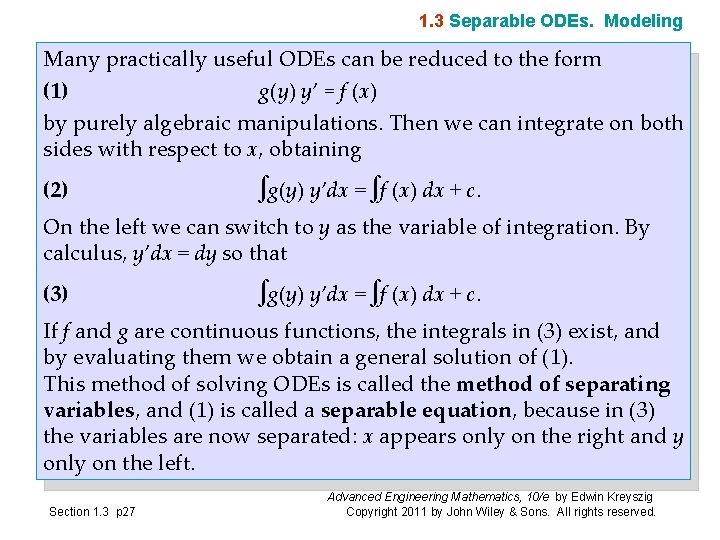
1. 3 Separable ODEs. Modeling Many practically useful ODEs can be reduced to the form (1) g(y) y’ = f (x) by purely algebraic manipulations. Then we can integrate on both sides with respect to x, obtaining (2) ∫g(y) y’dx = ∫f (x) dx + c. On the left we can switch to y as the variable of integration. By calculus, y’dx = dy so that (3) ∫g(y) y’dx = ∫f (x) dx + c. If f and g are continuous functions, the integrals in (3) exist, and by evaluating them we obtain a general solution of (1). This method of solving ODEs is called the method of separating variables, and (1) is called a separable equation, because in (3) the variables are now separated: x appears only on the right and y only on the left. Section 1. 3 p 27 Advanced Engineering Mathematics, 10/e by Edwin Kreyszig Copyright 2011 by John Wiley & Sons. All rights reserved.

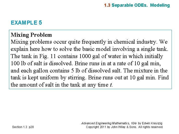
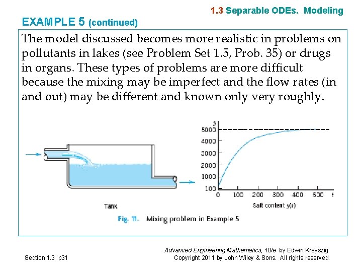
1. 3 Separable ODEs. Modeling EXAMPLE 5 Mixing Problem Mixing problems occur quite frequently in chemical industry. We explain here how to solve the basic model involving a single tank. The tank in Fig. 11 contains 1000 gal of water in which initially 100 lb of salt is dissolved. Brine runs in at a rate of 10 gal min, and each gallon contains 5 lb of dissolved salt. The mixture in the tank is kept uniform by stirring. Brine runs out at 10 gal min. Find the amount of salt in the tank at any time t. Section 1. 3 p 28 Advanced Engineering Mathematics, 10/e by Edwin Kreyszig Copyright 2011 by John Wiley & Sons. All rights reserved.

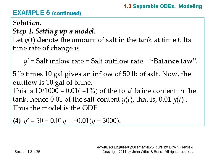
1. 3 Separable ODEs. Modeling EXAMPLE 5 (continued) Solution. Step 1. Setting up a model. Let y(t) denote the amount of salt in the tank at time t. Its time rate of change is y’ = Salt inflow rate = Salt outflow rate “Balance law”. 5 lb times 10 gal gives an inflow of 50 lb of salt. Now, the outflow is 10 gal of brine. This is 10/1000 = 0. 01( =1%) of the total brine content in the tank, hence 0. 01 of the salt content y(t), that is, 0. 01 y(t). Thus the model is the ODE (4) y’ = 50 − 0. 01 y = − 0. 01(y − 5000). Section 1. 3 p 29 Advanced Engineering Mathematics, 10/e by Edwin Kreyszig Copyright 2011 by John Wiley & Sons. All rights reserved.

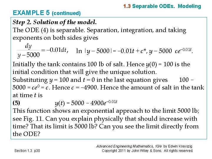
1. 3 Separable ODEs. Modeling EXAMPLE 5 (continued) Step 2. Solution of the model. The ODE (4) is separable. Separation, integration, and taking exponents on both sides gives ln |y − 5000|= − 0. 01 t + c*, y − 5000 ce− 0. 01 t. Initially the tank contains 100 lb of salt. Hence y(0) = 100 is the initial condition that will give the unique solution. Substituting y = 100 and t = 0 in the last equation gives 100 − 5000 = ce 0 = c. Hence c = − 4900. Hence the amount of salt in the tank at time t is (5) y(t) = 5000 − 4900 e− 0. 01 t This function shows an exponential approach to the limit 5000 lb; see Fig. 11. Can you explain physically that should increase with time? That its limit is 5000 lb? Can you see the limit directly from the ODE? Section 1. 3 p 30 Advanced Engineering Mathematics, 10/e by Edwin Kreyszig Copyright 2011 by John Wiley & Sons. All rights reserved.

EXAMPLE 5 (continued) 1. 3 Separable ODEs. Modeling The model discussed becomes more realistic in problems on pollutants in lakes (see Problem Set 1. 5, Prob. 35) or drugs in organs. These types of problems are more difficult because the mixing may be imperfect and the flow rates (in and out) may be different and known only very roughly. Section 1. 3 p 31 Advanced Engineering Mathematics, 10/e by Edwin Kreyszig Copyright 2011 by John Wiley & Sons. All rights reserved.

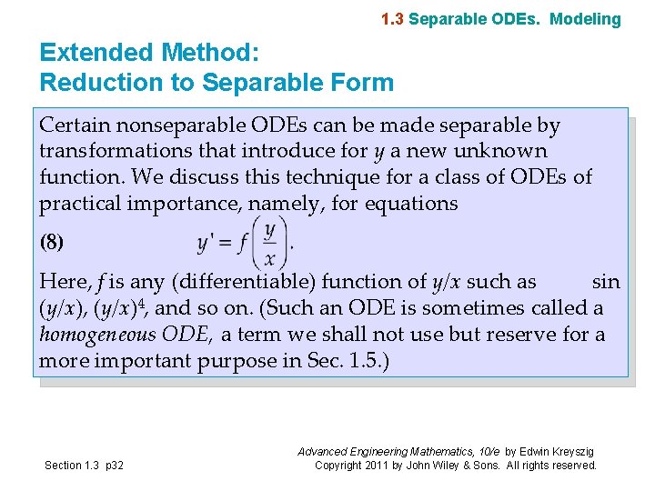
1. 3 Separable ODEs. Modeling Extended Method: Reduction to Separable Form Certain nonseparable ODEs can be made separable by transformations that introduce for y a new unknown function. We discuss this technique for a class of ODEs of practical importance, namely, for equations (8) Here, f is any (differentiable) function of y/x such as sin (y/x), (y/x)4, and so on. (Such an ODE is sometimes called a homogeneous ODE, a term we shall not use but reserve for a more important purpose in Sec. 1. 5. ) Section 1. 3 p 32 Advanced Engineering Mathematics, 10/e by Edwin Kreyszig Copyright 2011 by John Wiley & Sons. All rights reserved.

1. 3 Separable ODEs. Modeling Extended Method: Reduction to Separable Form (continued) The form of such an ODE suggests that we set y/x = u; thus, (9) y = ux and by product differentiation y’ = u’x + u. Substitution into y’ = f(y/x) then gives u’x + u = f (u) or u’x = f(u) − u. We see that if f(u) − u ≠ 0, this can be separated: (10) Section 1. 3 p 33 Advanced Engineering Mathematics, 10/e by Edwin Kreyszig Copyright 2011 by John Wiley & Sons. All rights reserved.

1. 4 Section 1. 4 p 34 Exact ODEs. Integrating Factors Advanced Engineering Mathematics, 10/e by Edwin Kreyszig Copyright 2011 by John Wiley & Sons. All rights reserved.

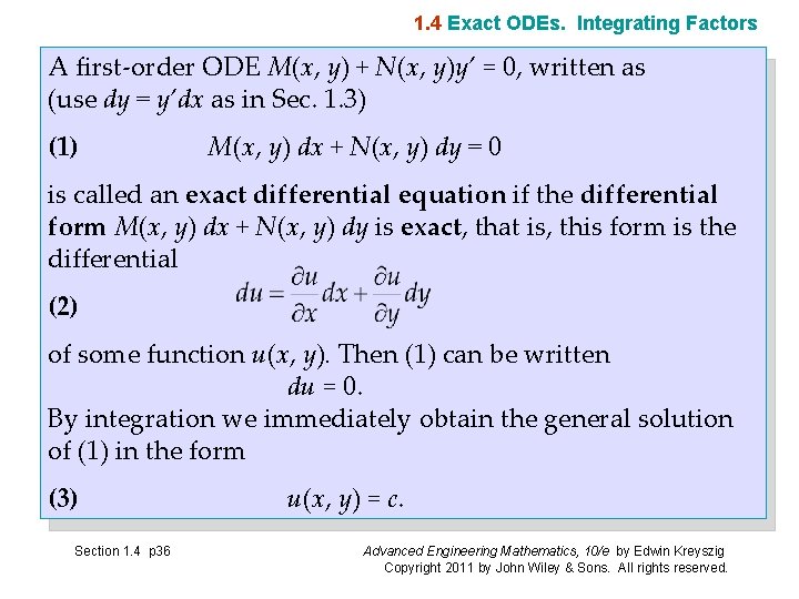
1. 4 Exact ODEs. Integrating Factors We recall from calculus that if a function has continuous partial derivatives, its differential (also called its total differential) is From this it follows that if then u(x, y) = const, du = 0. Section 1. 4 p 35 Advanced Engineering Mathematics, 10/e by Edwin Kreyszig Copyright 2011 by John Wiley & Sons. All rights reserved.

1. 4 Exact ODEs. Integrating Factors A first-order ODE M(x, y) + N(x, y)y’ = 0, written as (use dy = y’dx as in Sec. 1. 3) (1) M(x, y) dx + N(x, y) dy = 0 is called an exact differential equation if the differential form M(x, y) dx + N(x, y) dy is exact, that is, this form is the differential (2) of some function u(x, y). Then (1) can be written du = 0. By integration we immediately obtain the general solution of (1) in the form (3) Section 1. 4 p 36 u(x, y) = c. Advanced Engineering Mathematics, 10/e by Edwin Kreyszig Copyright 2011 by John Wiley & Sons. All rights reserved.

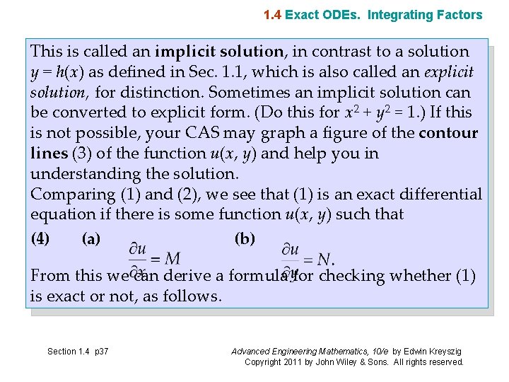
1. 4 Exact ODEs. Integrating Factors This is called an implicit solution, in contrast to a solution y = h(x) as defined in Sec. 1. 1, which is also called an explicit solution, for distinction. Sometimes an implicit solution can be converted to explicit form. (Do this for x 2 + y 2 = 1. ) If this is not possible, your CAS may graph a figure of the contour lines (3) of the function u(x, y) and help you in understanding the solution. Comparing (1) and (2), we see that (1) is an exact differential equation if there is some function u(x, y) such that (4) (a) (b) From this we can derive a formula for checking whether (1) is exact or not, as follows. Section 1. 4 p 37 Advanced Engineering Mathematics, 10/e by Edwin Kreyszig Copyright 2011 by John Wiley & Sons. All rights reserved.

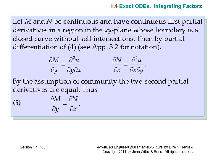
1. 4 Exact ODEs. Integrating Factors Let M and N be continuous and have continuous first partial derivatives in a region in the xy-plane whose boundary is a closed curve without self-intersections. Then by partial differentiation of (4) (see App. 3. 2 for notation), By the assumption of community the two second partial derivatives are equal. Thus (5) Section 1. 4 p 38 Advanced Engineering Mathematics, 10/e by Edwin Kreyszig Copyright 2011 by John Wiley & Sons. All rights reserved.

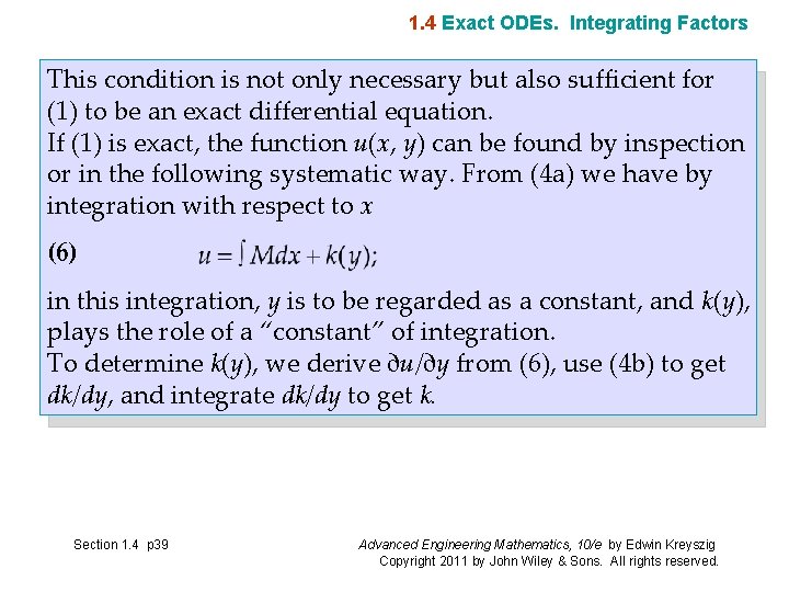
1. 4 Exact ODEs. Integrating Factors This condition is not only necessary but also sufficient for (1) to be an exact differential equation. If (1) is exact, the function u(x, y) can be found by inspection or in the following systematic way. From (4 a) we have by integration with respect to x (6) in this integration, y is to be regarded as a constant, and k(y), plays the role of a “constant” of integration. To determine k(y), we derive ∂u/∂y from (6), use (4 b) to get dk/dy, and integrate dk/dy to get k. Section 1. 4 p 39 Advanced Engineering Mathematics, 10/e by Edwin Kreyszig Copyright 2011 by John Wiley & Sons. All rights reserved.

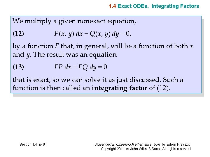
1. 4 Exact ODEs. Integrating Factors We multiply a given nonexact equation, (12) P(x, y) dx + Q(x, y) dy = 0, by a function F that, in general, will be a function of both x and y. The result was an equation (13) FP dx + FQ dy = 0 that is exact, so we can solve it as just discussed. Such a function is then called an integrating factor of (12). Section 1. 4 p 40 Advanced Engineering Mathematics, 10/e by Edwin Kreyszig Copyright 2011 by John Wiley & Sons. All rights reserved.

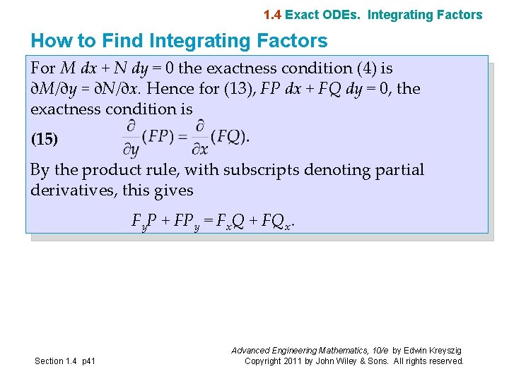
1. 4 Exact ODEs. Integrating Factors How to Find Integrating Factors For M dx + N dy = 0 the exactness condition (4) is ∂M/∂y = ∂N/∂x. Hence for (13), FP dx + FQ dy = 0, the exactness condition is (15) By the product rule, with subscripts denoting partial derivatives, this gives Fy. P + FPy = Fx. Q + FQx. Section 1. 4 p 41 Advanced Engineering Mathematics, 10/e by Edwin Kreyszig Copyright 2011 by John Wiley & Sons. All rights reserved.

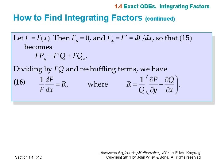
1. 4 Exact ODEs. Integrating Factors How to Find Integrating Factors (continued) Let F = F(x). Then Fy = 0, and Fx = F’ = d. F/dx, so that (15) becomes FPy = F’Q + FQx. Dividing by FQ and reshuffling terms, we have (16) Section 1. 4 p 42 Advanced Engineering Mathematics, 10/e by Edwin Kreyszig Copyright 2011 by John Wiley & Sons. All rights reserved.

1. 4 Exact ODEs. Integrating Factors Theorem Integrating Factor F(x) If (12) is such that the right side R of (16), depends only on x, then (12) has an integrating factor F = F(x), which is obtained by integrating (16) and taking exponents on both sides. (17) Note: (12) P(x, y) dx + Q(x, y) dy = 0, (16) Section 1. 4 p 43 Advanced Engineering Mathematics, 10/e by Edwin Kreyszig Copyright 2011 by John Wiley & Sons. All rights reserved.

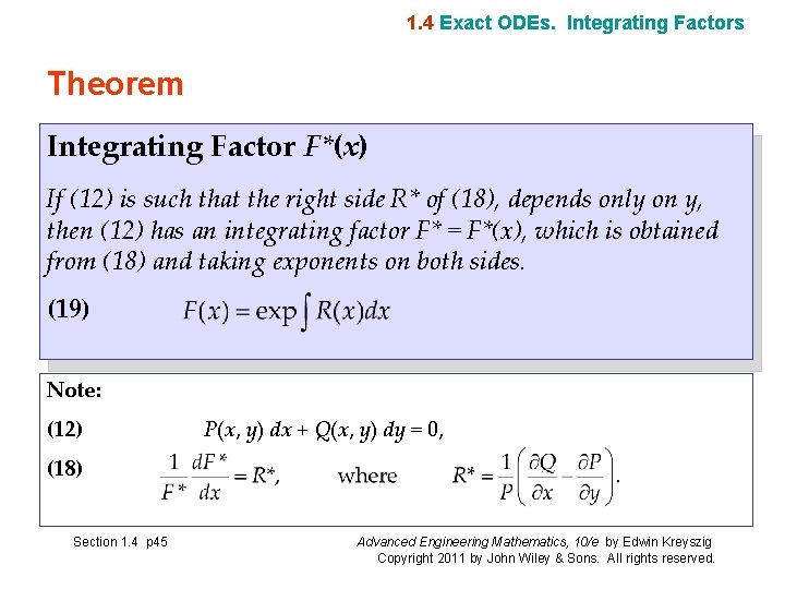
1. 4 Exact ODEs. Integrating Factors Similarly, if F* = F*(y), then instead of (16) we get (18) Section 1. 4 p 44 Advanced Engineering Mathematics, 10/e by Edwin Kreyszig Copyright 2011 by John Wiley & Sons. All rights reserved.

1. 4 Exact ODEs. Integrating Factors Theorem Integrating Factor F*(x) If (12) is such that the right side R* of (18), depends only on y, then (12) has an integrating factor F* = F*(x), which is obtained from (18) and taking exponents on both sides. (19) Note: (12) P(x, y) dx + Q(x, y) dy = 0, (18) Section 1. 4 p 45 Advanced Engineering Mathematics, 10/e by Edwin Kreyszig Copyright 2011 by John Wiley & Sons. All rights reserved.

1. 5 Linear ODEs. Bernoulli Equation. Population Dynamics Section 1. 5 p 46 Advanced Engineering Mathematics, 10/e by Edwin Kreyszig Copyright 2011 by John Wiley & Sons. All rights reserved.

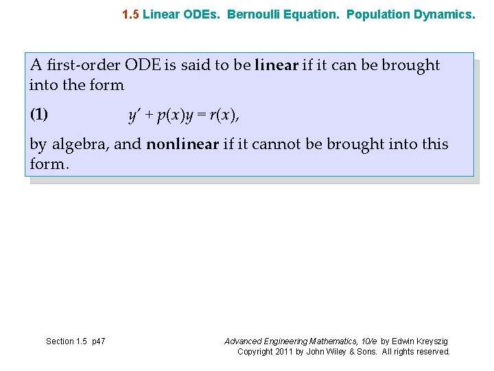
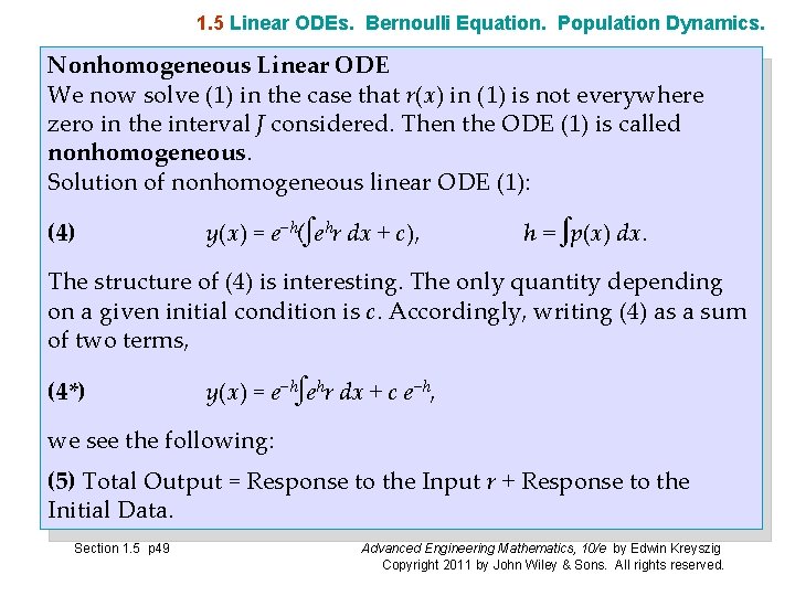
1. 5 Linear ODEs. Bernoulli Equation. Population Dynamics. A first-order ODE is said to be linear if it can be brought into the form (1) y’ + p(x)y = r(x), by algebra, and nonlinear if it cannot be brought into this form. Section 1. 5 p 47 Advanced Engineering Mathematics, 10/e by Edwin Kreyszig Copyright 2011 by John Wiley & Sons. All rights reserved.

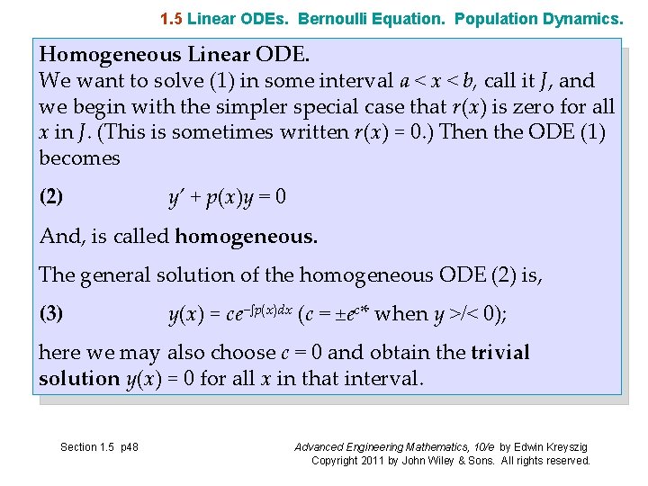
1. 5 Linear ODEs. Bernoulli Equation. Population Dynamics. Homogeneous Linear ODE. We want to solve (1) in some interval a < x < b, call it J, and we begin with the simpler special case that r(x) is zero for all x in J. (This is sometimes written r(x) = 0. ) Then the ODE (1) becomes (2) y’ + p(x)y = 0 And, is called homogeneous. The general solution of the homogeneous ODE (2) is, (3) y(x) = ce−∫p(x)dx (c = ±ec* when y >/< 0); here we may also choose c = 0 and obtain the trivial solution y(x) = 0 for all x in that interval. Section 1. 5 p 48 Advanced Engineering Mathematics, 10/e by Edwin Kreyszig Copyright 2011 by John Wiley & Sons. All rights reserved.

1. 5 Linear ODEs. Bernoulli Equation. Population Dynamics. Nonhomogeneous Linear ODE We now solve (1) in the case that r(x) in (1) is not everywhere zero in the interval J considered. Then the ODE (1) is called nonhomogeneous. Solution of nonhomogeneous linear ODE (1): (4) y(x) = e−h(∫ehr dx + c), h = ∫p(x) dx. The structure of (4) is interesting. The only quantity depending on a given initial condition is c. Accordingly, writing (4) as a sum of two terms, (4*) y(x) = e−h∫ehr dx + c e−h, we see the following: (5) Total Output = Response to the Input r + Response to the Initial Data. Section 1. 5 p 49 Advanced Engineering Mathematics, 10/e by Edwin Kreyszig Copyright 2011 by John Wiley & Sons. All rights reserved.

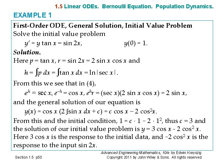
1. 5 Linear ODEs. Bernoulli Equation. Population Dynamics. EXAMPLE 1 First-Order ODE, General Solution, Initial Value Problem Solve the initial value problem y’ = y tan x = sin 2 x, y(0) = 1. Solution. Here p = tan x, r = sin 2 x = 2 sin x cos x and h = ∫p dx = ∫tan x dx = ln|sec x|. From this we see that in (4), eh = sec x, e−h = cos x, ehr = (sec x)(2 sin x cos x) = 2 sin x, and the general solution of our equation is y(x) = cos x (2 ∫sin x dx + c) = c cos x − 2 cos 2 x. From this and the initial condition, 1 = c · 1 − 2 · 12, thus c = 3 and the solution of our initial value problem is y = 3 cos x - 2 cos 2 x. Here 3 cos x is the response to the initial data, and − 2 cos 2 x is the response to the input sin 2 x. Section 1. 5 p 50 Advanced Engineering Mathematics, 10/e by Edwin Kreyszig Copyright 2011 by John Wiley & Sons. All rights reserved.

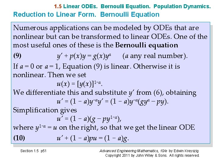
1. 5 Linear ODEs. Bernoulli Equation. Population Dynamics. Reduction to Linear Form. Bernoulli Equation Numerous applications can be modeled by ODEs that are nonlinear but can be transformed to linear ODEs. One of the most useful ones of these is the Bernoulli equation (9) y’ + p(x)y = g(x)ya (a any real number). If a = 0 or a = 1, Equation (9) is linear. Otherwise it is nonlinear. Then we set u(x) = [y(x)]1−a. We differentiate this and substitute y’ from (6), obtaining u’ = (1 − a)y−ay’ = (1 − a)y−a(gya − py). Simplification gives u’ = (1 − a)(g − py 1−a), where y 1−a = u on the right, so that we get the linear ODE (10) u’ + (1 − a)pu = (1 − a)g. Section 1. 5 p 51 Advanced Engineering Mathematics, 10/e by Edwin Kreyszig Copyright 2011 by John Wiley & Sons. All rights reserved.

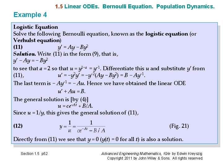
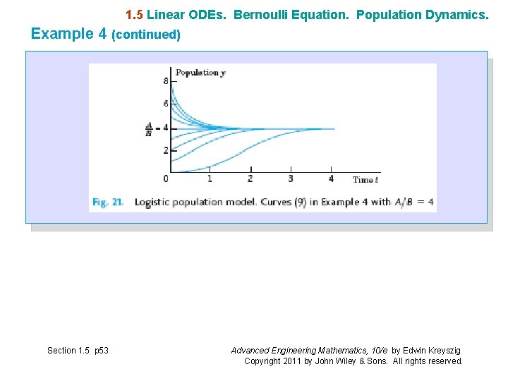
1. 5 Linear ODEs. Bernoulli Equation. Population Dynamics. Example 4 Logistic Equation Solve the following Bernoulli equation, known as the logistic equation (or Verhulst equation) (11) y’ = Ay − By 2 Solution. Write (11) in the form (9), that is, y’ − Ay = − By 2 to see that a = 2 so that u = y 1−a = y− 1. Differentiate this u and substitute y’ from (11), u’ = −y 2 y’ = −y− 2(Ay − By 2) = B − Ay− 1. The last term is − Ay− 1 = − Au. Hence we have obtained the linear ODE u’ + Au = B. The general solution is [by (4)] u = ce−At + B/A. Since u = 1/y, this gives the general solution of (11), (12) (Fig. 21) Directly from (11) we see that y = 0 (y(t) = 0 for all t) is also a solution. Section 1. 5 p 52 Advanced Engineering Mathematics, 10/e by Edwin Kreyszig Copyright 2011 by John Wiley & Sons. All rights reserved.

1. 5 Linear ODEs. Bernoulli Equation. Population Dynamics. Example 4 (continued) Section 1. 5 p 53 Advanced Engineering Mathematics, 10/e by Edwin Kreyszig Copyright 2011 by John Wiley & Sons. All rights reserved.

1. 5 Linear ODEs. Bernoulli Equation. Population Dynamics. We see that in the logistic equation (11) the independent variable t does not occur explicitly. An ODE y’ = f(t, y) in which t does not occur explicitly is of the form (13) y’ = f(y) and is called an autonomous ODE. Thus the logistic equation (11) is autonomous. Equation (10) has constant solutions, called equilibrium solutions or equilibrium points. These are determined by the zeros of f(y), because f(y) = 0 gives y’ = 0 by (13); hence y = const These zeros are known as critical points of (13). An equilibrium solution is called stable if solutions close to it for some t remain close to it for all further t. It is called unstable if solutions initially close to it do not remain close to it as t increases. Section 1. 5 p 54 Advanced Engineering Mathematics, 10/e by Edwin Kreyszig Copyright 2011 by John Wiley & Sons. All rights reserved.

1. 6 Section 1. 6 p 55 Orthogonal Trajectories. Optional Advanced Engineering Mathematics, 10/e by Edwin Kreyszig Copyright 2011 by John Wiley & Sons. All rights reserved.

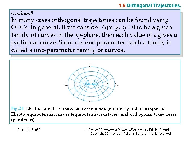
1. 6 Orthogonal Trajectories. An important type of problem in physics or geometry is to find a family of curves that intersect a given family of curves at right angles. The new curves are called orthogonal trajectories of the given curves (and conversely). Examples are curves of equal temperature (isotherms) and curves of heat flow, curves of equal altitude (contour lines) on a map and curves of steepest descent on that map, curves of equal potential (equipotential curves, curves of equal voltage-the ellipses in Fig. 24, next slide) and curves of electric force (the parabolas in Fig. 24). Here the angle of intersection between two curves is defined to be the angle between the tangents of the curves at the intersection point. Orthogonal is another word for perpendicular. Section 1. 6 p 56 Advanced Engineering Mathematics, 10/e by Edwin Kreyszig Copyright 2011 by John Wiley & Sons. All rights reserved.

1. 6 Orthogonal Trajectories. (continued) In many cases orthogonal trajectories can be found using ODEs. In general, if we consider G(x, y, c) = 0 to be a given family of curves in the xy-plane, then each value of c gives a particular curve. Since c is one parameter, such a family is called a one-parameter family of curves. Fig. 24 Electrostatic field between two ellipses (elliptic cylinders in space): Elliptic equipotential curves (equipotential surfaces) and orthogonal trajectories (parabolas) Section 1. 6 p 57 Advanced Engineering Mathematics, 10/e by Edwin Kreyszig Copyright 2011 by John Wiley & Sons. All rights reserved.

1. 7 Existence and Uniqueness of Solutions for Initial Value Problems Section 1. 7 p 58 Advanced Engineering Mathematics, 10/e by Edwin Kreyszig Copyright 2011 by John Wiley & Sons. All rights reserved.

1. 7 Existence and Uniqueness of Solutions for Initial Value Problems Problem of Existence Under what conditions does an initial value problem of the form (1) have at least one solution (hence one or several solutions)? Problem of Uniqueness Under what conditions does that problem have at most one solution (hence excluding the case that is has more than one solution)? Section 1. 7 p 59 Advanced Engineering Mathematics, 10/e by Edwin Kreyszig Copyright 2011 by John Wiley & Sons. All rights reserved.

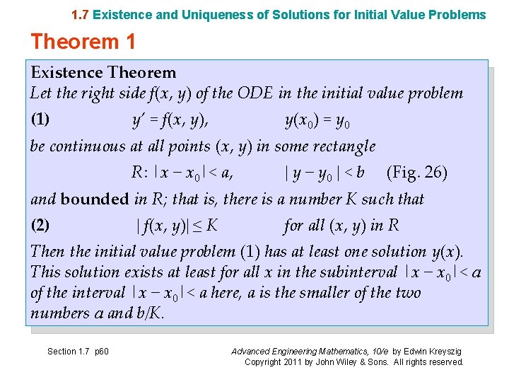
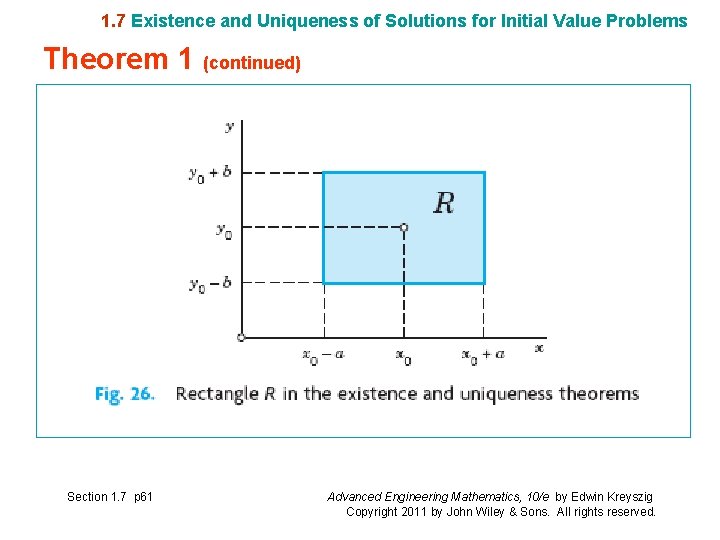
1. 7 Existence and Uniqueness of Solutions for Initial Value Problems Theorem 1 Existence Theorem Let the right side f(x, y) of the ODE in the initial value problem (1) y’ = f(x, y), y(x 0) = y 0 be continuous at all points (x, y) in some rectangle R: |x − x 0|< a, | y − y 0 | < b (Fig. 26) and bounded in R; that is, there is a number K such that (2) | f(x, y)| ≤ K for all (x, y) in R Then the initial value problem (1) has at least one solution y(x). This solution exists at least for all x in the subinterval |x − x 0|< a of the interval |x − x 0|< a here, a is the smaller of the two numbers a and b/K. Section 1. 7 p 60 Advanced Engineering Mathematics, 10/e by Edwin Kreyszig Copyright 2011 by John Wiley & Sons. All rights reserved.

1. 7 Existence and Uniqueness of Solutions for Initial Value Problems Theorem 1 (continued) Section 1. 7 p 61 Advanced Engineering Mathematics, 10/e by Edwin Kreyszig Copyright 2011 by John Wiley & Sons. All rights reserved.

1. 7 Existence and Uniqueness of Solutions for Initial Value Problems Theorem 2 Uniqueness Theorem Let f and its partial derivative fy = ∂f/∂y be continuous for all (x, y) in the rectangle R (Fig. 26) and bounded, say, (3) (a) |f (x, y)| ≤ K, (b) |f y(x, y)| ≤ M for all (x, y) in R. Then the initial value problem (1) has at most one solution y(x). Thus, by Theorem 1, the problem has precisely one solution. This solution exists at least for all x in that subinterval |x − x 0|< a. Section 1. 7 p 62 Advanced Engineering Mathematics, 10/e by Edwin Kreyszig Copyright 2011 by John Wiley & Sons. All rights reserved.

1 First-Order ODEs SUMMARY OF CHAPTER Section 1. Summary p 63 Advanced Engineering Mathematics, 10/e by Edwin Kreyszig Copyright 2011 by John Wiley & Sons. All rights reserved.

SUMMARY OF CHAPTER 1 First-Order ODEs This chapter concerns ordinary differential equations (ODEs) of first order and their applications. These are equations of the form (1) F(x, y, y’) = 0 or in explicit form y’ = f(x, y) involving the derivative y’ = dy/dx of an unknown function y, given functions of x, and, perhaps, y itself. If the independent variable x is time, we denote it by t. In Sec. 1. 1 we explained the basic concepts and the process of modeling, that is, of expressing a physical or other problem in some mathematical form and solving it. Then we discussed the method of direction fields (See. 1. 2), solution methods and models (Sees. 1. 3– 1. 6), and, finally, ideas on existence and uniqueness of solutions (Sec. 1. 7). Section 1. Summary p 64 Advanced Engineering Mathematics, 10/e by Edwin Kreyszig Copyright 2011 by John Wiley & Sons. All rights reserved.

SUMMARY OF CHAPTER 1 First-Order ODEs (continued 1) A first-order ODE usually has a general solution, that is, a solution involving an arbitrary constant, which we denote by c. In applications we usually have to find a unique solution by determining a value of c from an initial condition y(x 0) = y 0. Together with the ODE this is called an initial value problem (2) y’ = f(x, y) y(x 0) = y 0 (x 0, y 0 given numbers) and its solution is a particular solution of the ODE. Geometrically, a general solution represents a family of curves, which can be graphed by using direction fields (Sec. 1. 2). And each particular solution corresponds to one of these curves. Section 1. Summary p 65 Advanced Engineering Mathematics, 10/e by Edwin Kreyszig Copyright 2011 by John Wiley & Sons. All rights reserved.

SUMMARY OF CHAPTER 1 First-Order ODEs (continued 2) A separable ODE is one that we can put into the form (3) g(y) dy = f (x) dx (Sec. 1. 3) by algebraic manipulations (possibly combined with transformations, such as y/x = u) and solve by integrating on both sides. An exact ODE is of the form (4) M(x, y) dx + N(x, y) dy = 0 (Sec. 1. 4) where M dx + N dy is the differential du = ux dx + uy dy of a function u(x, y), so that from du = 0 we immediately get the implicit general solution u(x, y) = c. This method extends to nonexact ODEs that can be made exact by multiplying them by some function F(x, y, ), called an integrating factor (Sec. 1. 4). Section 1. Summary p 66 Advanced Engineering Mathematics, 10/e by Edwin Kreyszig Copyright 2011 by John Wiley & Sons. All rights reserved.

SUMMARY OF CHAPTER 1 First-Order ODEs Linear ODEs (5) y’ + p(x)y = r(x) are very important. Their solutions are given by the integral formula (4). Sec. 1. 5. Certain nonlinear ODEs can be transformed to linear form in terms of new variables. This holds for the Bernoulli equation y’ + p(x)y = g(x)ya (Sec. 1. 5). Applications and modeling are discussed throughout the chapter, in particular in Secs. 1. 1, 1. 3, 1. 5 (population dynamics, etc. ), and 1. 6 (trajectories). Picard’s existence and uniqueness theorems are explained in Sec. 1. 7 (and Picard’s iteration in Problem Set 1. 7). Numeric methods for first-order ODEs can be studied in Secs. 21. 1 and 21. 2 immediately after this chapter, as indicated in the chapter opening. (continued 3) Section 1. Summary p 67 Advanced Engineering Mathematics, 10/e by Edwin Kreyszig Copyright 2011 by John Wiley & Sons. All rights reserved.