Part 5 Queueing Models CSC 446546 Agenda 1

Part 5: Queueing Models CSC 446/546

Agenda 1. The Purpose 2. Characteristics of Queues Systems 3. Queueing Notations 4. Long-Run Measures 5. Steady-State Behavior of Infinite-Population Markovian Models 6. Steady-State Behavior of Finite-Population Markovian Models 7. Final Summary CSC 446/546

1. The Purpose (1): Queueing System Examples CSC 446/546 2

1. The Purpose (2) n. Simulation is often used in the analysis of queueing models. n. Queueing models provide the analyst with a powerful tool for designing and evaluating the performance of queueing systems. Discuss some well-known models (NOT development of queueing theories) n CSC 446/546 3

2. Characteristics of Queueing Systems (1): Key Elements Key elements of queueing systems: • Customer: refers to anything that arrives at a facility and requires service, e. g. , people, machines, trucks, emails. • Server: refers to any resource that provides the requested service, e. g. , repair persons, retrieval machines, runways at airport. Waiting Line Server(s) Customer Arrivals Calling Population Arrival Process CSC 446/546 System Capacity Queue Behavior Queue Discipline Service Times Service Mechanisms 4

2. Characteristics of Queueing Systems (2): Calling Population Calling population: the population of potential customers, may be assumed to be finite or infinite. • Finite population model: if arrival rate depends on the number of customers being served and waiting, e. g. , model of one corporate jet, if it is being repaired, the repair arrival rate becomes zero. • Infinite population model: if arrival rate is not affected by the number of customers being served and waiting, e. g. , systems with large population of potential customers. CSC 446/546 5

2. Characteristics of Queueing Systems (3): System Capacity: a limit on the number of customers that may be in the waiting line or system. • Limited capacity, e. g. , an automatic car wash only has room for 10 cars to wait in line to enter the mechanism. • Unlimited capacity, e. g. , concert ticket sales with no limit on the number of people allowed to wait to purchase tickets. CSC 446/546 6

2. Characteristics of Queueing Systems (4): Arrival Process (1) For infinite-population models: • Usually characterized in terms of inter-arrival times of successive customers. Arrivals may occur at random or scheduled times • Random arrivals: inter-arrival times usually characterized by a probability distribution. – Most important model: Poisson arrival process (with rate ), where An represents the inter-arrival time between customer n-1 and customer n, and is exponentially distributed (with mean 1/ ). • Scheduled arrivals: inter-arrival times can be constant or constant plus or minus a small random amount (jitter) to represent early or late arrivals. – e. g. , patients to a physician or scheduled airline flight arrivals to an airport. • At least one customer is assumed to always be present, so the server is never idle, e. g. , sufficient raw material for a machine. CSC 446/546 7

2. Characteristics of Queueing Systems (4): Arrival Process (2) For finite-population models: • Define customer as “pending” when the customer is outside the queueing system, e. g. , machine-repair problem: a machine is “pending” when it is operating, it becomes “not pending” the instant it demands service form the repairman. • Define “runtime” of a customer as the length of time from departure from the queueing system until that customer’s next arrival to the queue, e. g. , machine-repair problem, machines are customers and a runtime is time to failure. • Let A 1(i), A 2(i), … be the successive runtimes of customer i, and S 1(i), S 2(i) be the corresponding successive system times: that is Sn(i) is the total time spent in the system by customer i during the nth visit. CSC 446/546 8

2. Characteristics of Queueing Systems (4): Arrival Process (3) Finite Population Models • The total arrival process is the superposition of the arrival times of all customers. • One important application of finite models is the machine-repair problem. Machines are the customers and runtime is time to failure. When a machine fails, it “arrives” at the queueing system and remains there until it is served. Time to failure is chracterized by exponential, Weibull and Gamma distributions. CSC 446/546 9

2. Characteristics of Queueing Systems (5): Queue Behavior and Queue Discipline Queue behavior: refers to the actions of customers while in a queue waiting for service to begin, for example: • Balk: leave when they see that the line is too long, • Renege: leave after being in the line when its moving too slowly, • Jockey: move from one line to a shorter line. Queue discipline: refers to the logical ordering of customers in a queue that determines which customer is chosen for service when a server becomes free, for example: • • • First-in-first-out (FIFO) Last-in-first-out (LIFO) Service in random order (SIRO) Shortest processing time first (SPT) Service according to priority (PR). (e. g. , type, class, priority) CSC 446/546 10

2. Characteristics of Queueing Systems (6): Service Times and Service Mechanism (1) Service times of successive arrivals are denoted by S 1, S 2, S 3, …… • May be constant or random. • {S 1, S 2, S 3, …} is usually characterized as a sequence of independent and identically distributed random variables, e. g. , exponential, Weibull, gamma, lognormal, and truncated normal distribution. • Sometimes, services are identically distributed for all customers of a given type or class or priority, where as customers of different types might have completely different service-time distributions • In some systems, service times depend upon the time of the day or upon the length of waiting line (e. g. , servers might work faster than usual if waiting times are long, effectively reducing service times) CSC 446/546 11

2. Characteristics of Queueing Systems (6): Service Times and Service Mechanism (2) A queueing system consists of a number of service centers and interconnected queues. • Each service center consists of some number of servers, c, working in parallel • upon getting to the head of the line, a customer takes the 1 st available server. • Parallel service mechanisms are either single server (c=1), multiple server (1<c< ), or unlimited servers (c= ) – A self service facility is usually characterized by an unlimited number of servers CSC 446/546 12

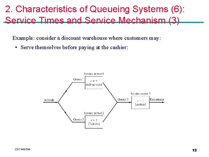
2. Characteristics of Queueing Systems (6): Service Times and Service Mechanism (3) Example: consider a discount warehouse where customers may: • Serve themselves before paying at the cashier: CSC 446/546 13

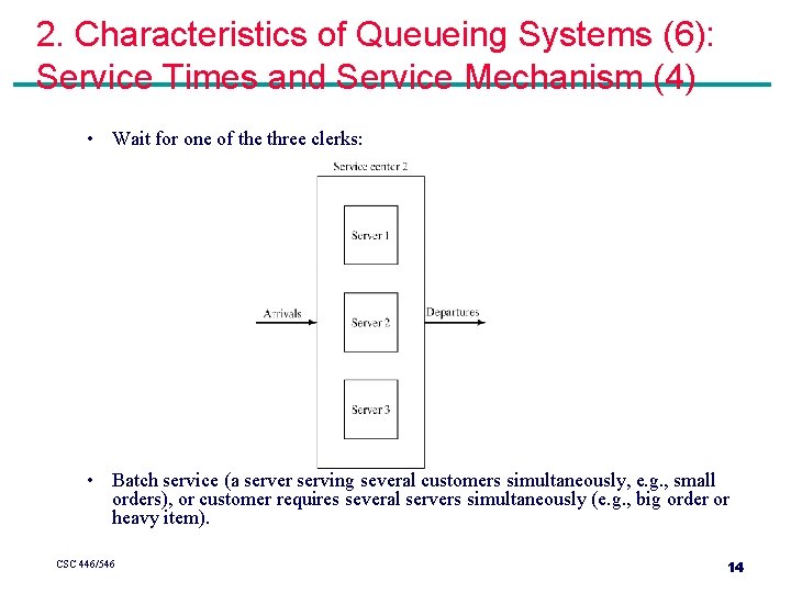
2. Characteristics of Queueing Systems (6): Service Times and Service Mechanism (4) • Wait for one of the three clerks: • Batch service (a server serving several customers simultaneously, e. g. , small orders), or customer requires several servers simultaneously (e. g. , big order or heavy item). CSC 446/546 14

3. Queueing Notation (1) Recognizing the diversity of queueing systems, Kendall proposed a notational system in 1953 that has been widely adopted. A notation system for parallel server queues: A/B/c/N/K • A represents the inter-arrival-time distribution, • B represents the service-time distribution, • c represents the number of parallel servers, N represents the system capacity, • K represents the size of the calling population. Common symbols for A and B include M (exponential), D (constant or deterministic), Ek (for Erlang order k), PH (Phase-type), H (hyperexponential), G (arbitrary or general), and GI (general independent). CSC 446/546 15

3. Queueing Notation (2) Examples: • M/M/1 (also M/M/1/ / ) indicates a single-server that has unlimited queue capacity and an infinite population model. The interarrivals and service times are exponentially distributed. – When N and K are infinite, they are often dropped from the notation • G/G/1/5/5 represents a queueing system with general (or arbitrary) interarrival and service distribution with single server, with a queue capacity of 5 and finite population model of size 5 – General models are used to solve the queue system with no particular distribution in mind – Very useful as the final results can be obtained by plugging in the values of specific distributions CSC 446/546 16

3. Queueing Notation (3) Primary performance measures of queueing systems: § Pn: steady-state probability of having n customers in system, § Pn(t): probability of n customers in system at time t, § : arrival rate, § e: effective arrival rate, § : service rate of one server, § : server utilization, § An: inter-arrival time between customers n-1 and n § Sn: service time of the nth arriving customer, § Wn: total time spent in system by the nth arriving customer, § Wn. Q: total time spent in the waiting line by customer n, § L(t): the number of customers in system at time t, § LQ(t): the number of customers in queue at time t, § L: long-run time-average number of customers in system, § LQ: long-run time-average number of customers in queue, § w: long-run average time spent in system per customer, § w. Q: long-run average time spent in queue per customer. CSC 446/546 17

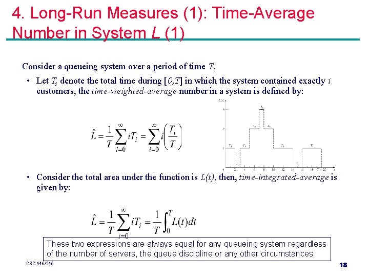
4. Long-Run Measures (1): Time-Average Number in System L (1) Consider a queueing system over a period of time T, • Let Ti denote the total time during [0, T] in which the system contained exactly i customers, the time-weighted-average number in a system is defined by: • Consider the total area under the function is L(t), then, time-integrated-average is given by: These two expressions are always equal for any queueing system regardless of the number of servers, the queue discipline or any other circumstances CSC 446/546 18

4. Long-Run Measures (1): Time-Average Number in System L (2) Many queueing systems exhibit long-run stability in terms of their average performance. For such systems, as time T gets large, the observed time-average number in the system approaches a limiting value L, called long-run time-average. The long-run time-average # in system L, with probability 1: The estimator is said to be strongly consistent for L. If simulation run length T is sufficiently long, the estimator becomes arbitrarily close to L. Unfortunately for T < , it depends on the initial condition at t=0. (Reason to do multiple simulation runs!!) CSC 446/546 19

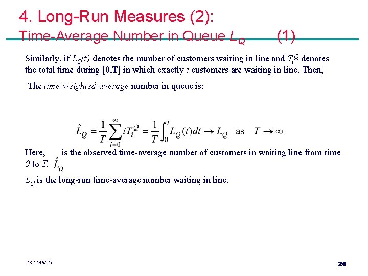
4. Long-Run Measures (2): Time-Average Number in Queue LQ (1) Similarly, if LQ(t) denotes the number of customers waiting in line and Ti. Q denotes the total time during [0, T] in which exactly i customers are waiting in line. Then, The time-weighted-average number in queue is: Here, 0 to T. is the observed time-average number of customers in waiting line from time LQ is the long-run time-average number waiting in line. CSC 446/546 20

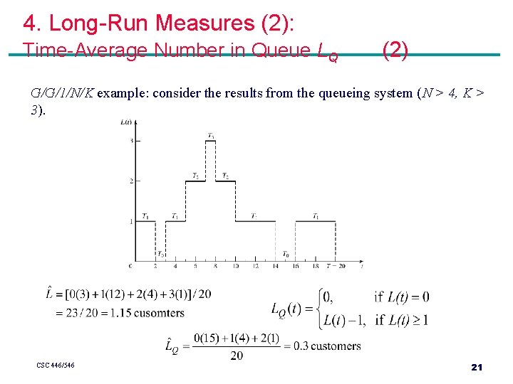
4. Long-Run Measures (2): Time-Average Number in Queue LQ (2) G/G/1/N/K example: consider the results from the queueing system (N > 4, K > 3). CSC 446/546 21

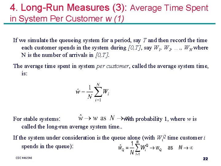
4. Long-Run Measures (3): Average Time Spent in System Per Customer w (1) If we simulate the queueing system for a period, say T and then record the time each customer spends in the system during [0, T], say W 1, W 2, …. , WN where N is the number of arrivals in [0, T]. The average time spent in system per customer, called the average system time, is: For stable systems: with probability 1, where w is called the long-run average system time. . If the system under consideration is the queue alone (with Wi. Q time customer i spends in the queue): CSC 446/546 22

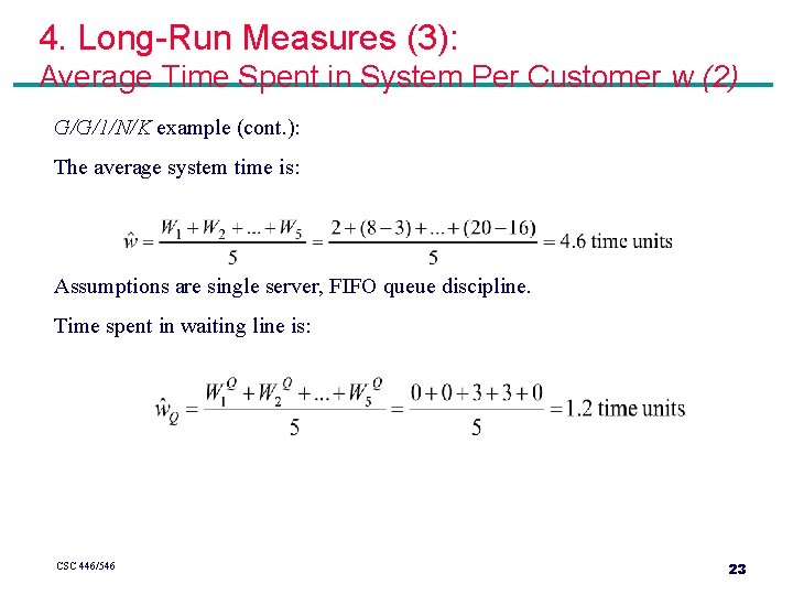
4. Long-Run Measures (3): Average Time Spent in System Per Customer w (2) G/G/1/N/K example (cont. ): The average system time is: Assumptions are single server, FIFO queue discipline. Time spent in waiting line is: CSC 446/546 23

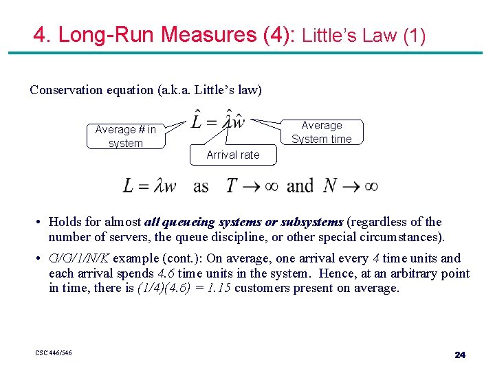
4. Long-Run Measures (4): Little’s Law (1) Conservation equation (a. k. a. Little’s law) Average # in system Average System time Arrival rate • Holds for almost all queueing systems or subsystems (regardless of the number of servers, the queue discipline, or other special circumstances). • G/G/1/N/K example (cont. ): On average, one arrival every 4 time units and each arrival spends 4. 6 time units in the system. Hence, at an arbitrary point in time, there is (1/4)(4. 6) = 1. 15 customers present on average. CSC 446/546 24

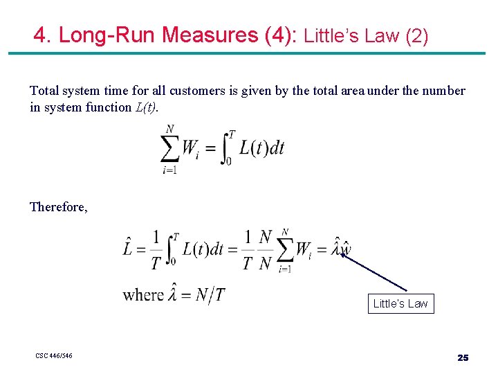
4. Long-Run Measures (4): Little’s Law (2) Total system time for all customers is given by the total area under the number in system function L(t). Therefore, Little’s Law CSC 446/546 25

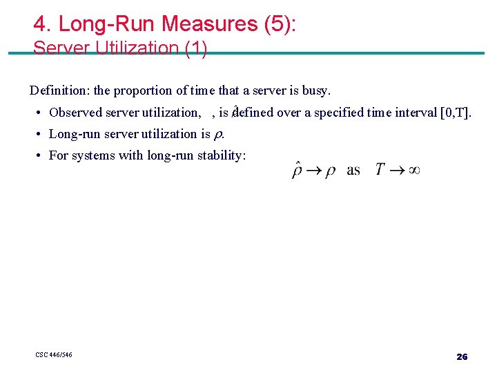
4. Long-Run Measures (5): Server Utilization (1) Definition: the proportion of time that a server is busy. • Observed server utilization, , is defined over a specified time interval [0, T]. • Long-run server utilization is . • For systems with long-run stability: CSC 446/546 26

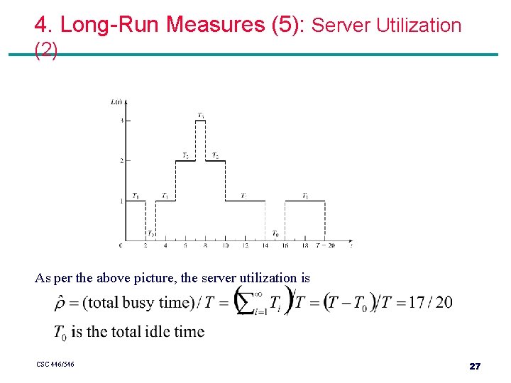
4. Long-Run Measures (5): Server Utilization (2) As per the above picture, the server utilization is CSC 446/546 27

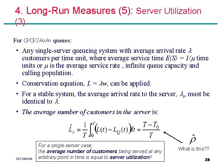
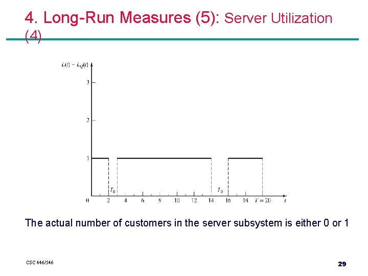
4. Long-Run Measures (5): Server Utilization (3) For G/G/1/∞/∞ queues: • Any single-server queueing system with average arrival rate customers per time unit, where average service time E(S) = 1/ time units or is the average service rate , infinite queue capacity and calling population. • Conservation equation, L = w, can be applied. • For a stable system, the average arrival rate to the server, s, must be identical to . • The average number of customers in the server is: CSC 446/546 For a single-server case, the average number of customers being served at any arbitrary point in time is equal to server utilization!! What is this? ? 28

4. Long-Run Measures (5): Server Utilization (4) The actual number of customers in the server subsystem is either 0 or 1 CSC 446/546 29

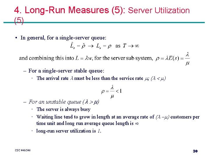
4. Long-Run Measures (5): Server Utilization (5) • In general, for a single-server queue: – For a single-server stable queue: · The arrival rate must be less than the service rate ; ( < ) – For an unstable queue ( > ) · The server is always busy · Waiting line tend to grow in length at an average rate of ( - ) customers per time unit and long run average queue length is · long-run server utilization is 1. CSC 446/546 30

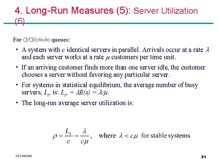
4. Long-Run Measures (5): Server Utilization (6) For G/G/c/∞/∞ queues: • A system with c identical servers in parallel. Arrivals occur at a rate and each server works at a rate customers per time unit. • If an arriving customer finds more than one server idle, the customer chooses a server without favoring any particular server. • For systems in statistical equilibrium, the average number of busy servers, Ls, is: Ls, = E(s) = /. • The long-run average server utilization is: CSC 446/546 31

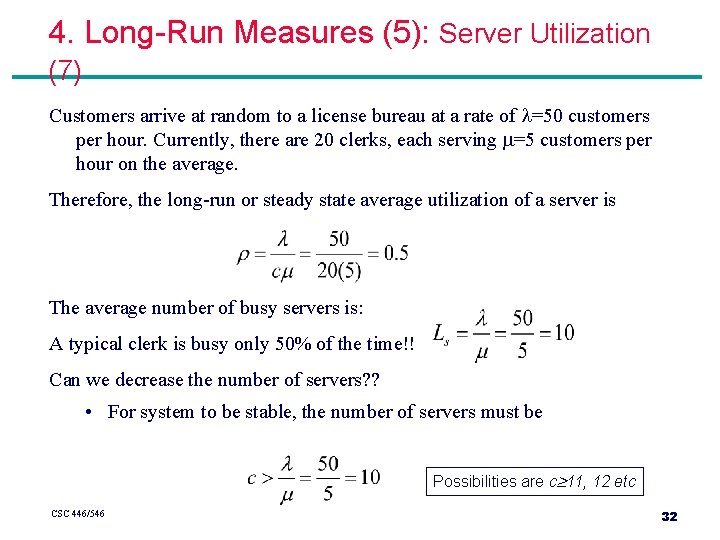
4. Long-Run Measures (5): Server Utilization (7) Customers arrive at random to a license bureau at a rate of =50 customers per hour. Currently, there are 20 clerks, each serving =5 customers per hour on the average. Therefore, the long-run or steady state average utilization of a server is The average number of busy servers is: A typical clerk is busy only 50% of the time!! Can we decrease the number of servers? ? • For system to be stable, the number of servers must be Possibilities are c 11, 12 etc CSC 446/546 32

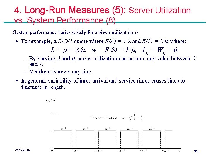
4. Long-Run Measures (5): Server Utilization vs. System Performance (8) System performance varies widely for a given utilization . • For example, a D/D/1 queue where E(A) = 1/ and E(S) = 1/ , where: L = = / , w = E(S) = 1/ , LQ = WQ = 0. – By varying and , server utilization can assume any value between 0 and 1. – Yet there is never any line. • In general, variability of inter-arrival and service times causes lines to fluctuate in length. CSC 446/546 33

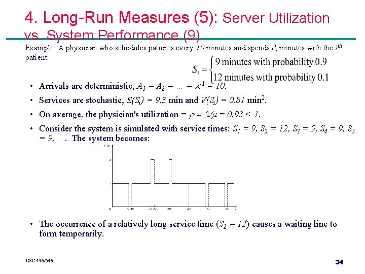
4. Long-Run Measures (5): Server Utilization vs. System Performance (9) Example: A physician who schedules patients every 10 minutes and spends Si minutes with the ith patient: • Arrivals are deterministic, A 1 = A 2 = … = -1 = 10. • Services are stochastic, E(Si) = 9. 3 min and V(Si) = 0. 81 min 2. • On average, the physician's utilization = = / = 0. 93 < 1. • Consider the system is simulated with service times: S 1 = 9, S 2 = 12, S 3 = 9, S 4 = 9, S 5 = 9, …. The system becomes: • The occurrence of a relatively long service time (S 2 = 12) causes a waiting line to form temporarily. CSC 446/546 34

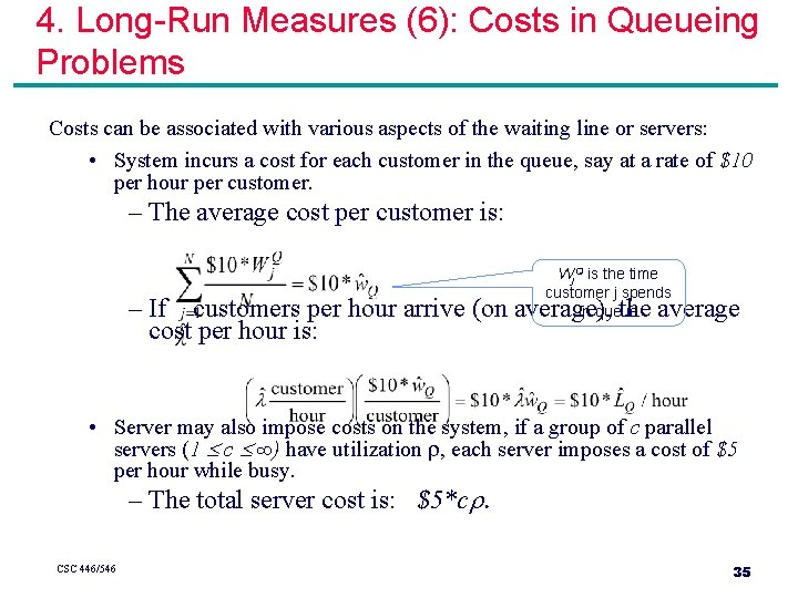
4. Long-Run Measures (6): Costs in Queueing Problems Costs can be associated with various aspects of the waiting line or servers: • System incurs a cost for each customer in the queue, say at a rate of $10 per hour per customer. – The average cost per customer is: Wj. Q is the time customer j spends in queue – If customers per hour arrive (on average), the average cost per hour is: • Server may also impose costs on the system, if a group of c parallel servers (1 £ c £ ∞) have utilization , each server imposes a cost of $5 per hour while busy. – The total server cost is: $5*c. CSC 446/546 35

5. Steady-State Behavior of Infinite. Population Markovian Models (1) Markovian models: exponential-distribution arrival process (mean arrival rate = ). Service times may be exponentially distributed (M) or arbitrary (G). A queueing system is in statistical equilibrium if the probability that the system is in a given state is not time dependent: P( L(t) = n ) = Pn(t) = Pn. Mathematical models in this chapter can be used to obtain approximate results even when the model assumptions do not strictly hold (as a rough guide). Simulation can be used for more refined analysis (more faithful representation for complex systems). CSC 446/546 36

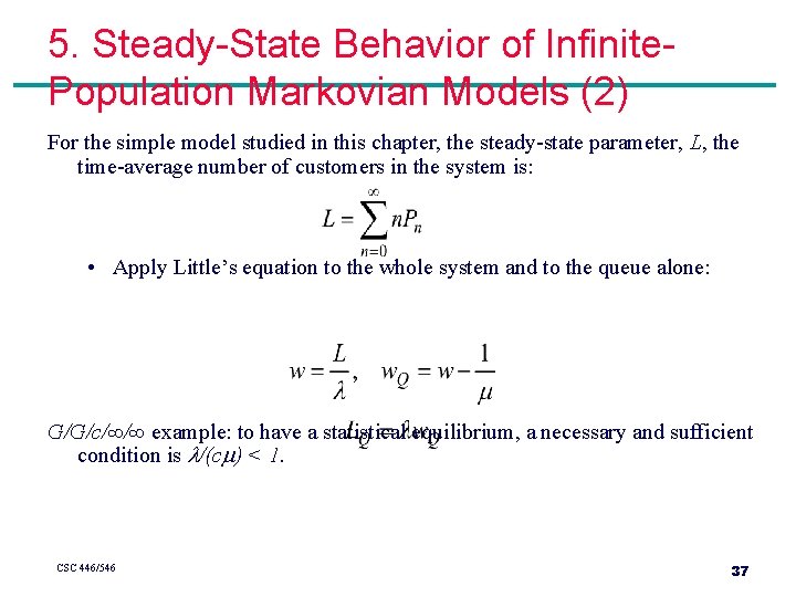
5. Steady-State Behavior of Infinite. Population Markovian Models (2) For the simple model studied in this chapter, the steady-state parameter, L, the time-average number of customers in the system is: • Apply Little’s equation to the whole system and to the queue alone: G/G/c/∞/∞ example: to have a statistical equilibrium, a necessary and sufficient condition is /(c ) < 1. CSC 446/546 37

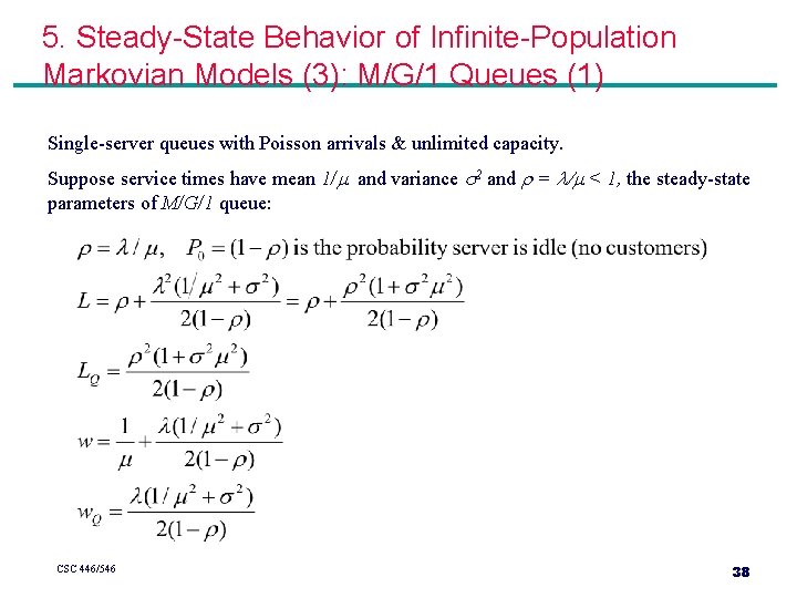
5. Steady-State Behavior of Infinite-Population Markovian Models (3): M/G/1 Queues (1) Single-server queues with Poisson arrivals & unlimited capacity. Suppose service times have mean 1/ and variance s 2 and = / < 1, the steady-state parameters of M/G/1 queue: CSC 446/546 38

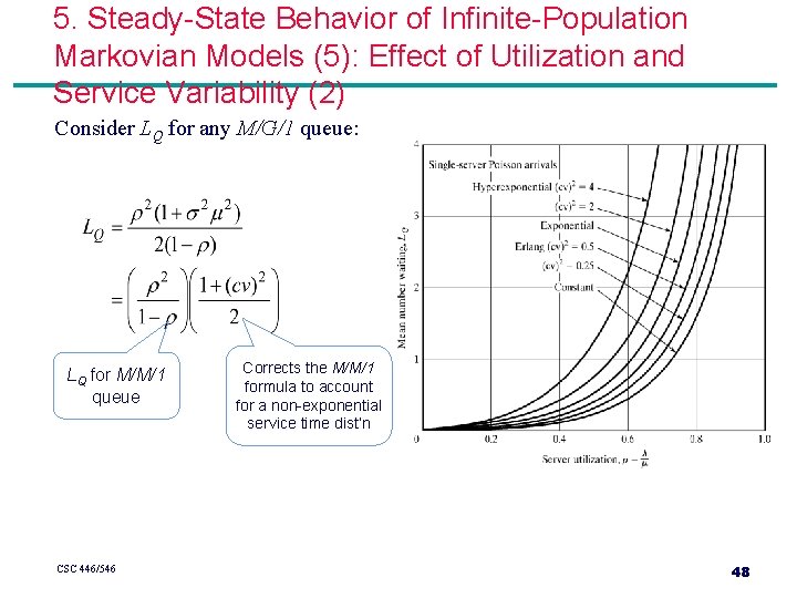
5. Steady-State Behavior of Infinite-Population Markovian Models (3): M/G/1 Queues (2) • No simple expression for the steady-state probabilities P 0, P 1, … • L – LQ = is the time-average number of customers being served. • Average length of queue, LQ, can be rewritten as: – If and are held constant, LQ depends on the variability, s 2, of the service times. CSC 446/546 39

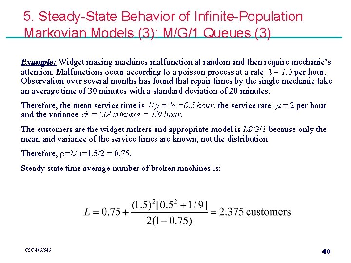
5. Steady-State Behavior of Infinite-Population Markovian Models (3): M/G/1 Queues (3) Example: Widget making machines malfunction at random and then require mechanic’s attention. Malfunctions occur according to a poisson process at a rate = 1. 5 per hour. Observation over several months has found that repair times by the single mechanic take an average time of 30 minutes with a standard deviation of 20 minutes. Therefore, the mean service time is 1/ = ½ =0. 5 hour, the service rate = 2 per hour and the variance s 2 = 202 minutes = 1/9 hour. The customers are the widget makers and appropriate model is M/G/1 because only the mean and variance of the service times are known, not the distribution Therefore, = / =1. 5/2 = 0. 75. Steady state time average number of broken machines is: CSC 446/546 40

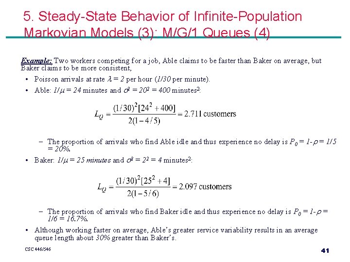
5. Steady-State Behavior of Infinite-Population Markovian Models (3): M/G/1 Queues (4) Example: Two workers competing for a job, Able claims to be faster than Baker on average, but Baker claims to be more consistent, • Poisson arrivals at rate = 2 per hour (1/30 per minute). • Able: 1/ = 24 minutes and s 2 = 202 = 400 minutes 2: – The proportion of arrivals who find Able idle and thus experience no delay is P 0 = 1 - = 1/5 = 20%. • Baker: 1/ = 25 minutes and s 2 = 22 = 4 minutes 2: – The proportion of arrivals who find Baker idle and thus experience no delay is P 0 = 1 - = 1/6 = 16. 7%. • Although working faster on average, Able’s greater service variability results in an average queue length about 30% greater than Baker’s. CSC 446/546 41

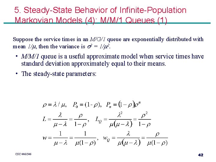
5. Steady-State Behavior of Infinite-Population Markovian Models (4): M/M/1 Queues (1) Suppose the service times in an M/G/1 queue are exponentially distributed with mean 1/ , then the variance is s 2 = 1/ 2. • M/M/1 queue is a useful approximate model when service times have standard deviation approximately equal to their means. • The steady-state parameters: CSC 446/546 42

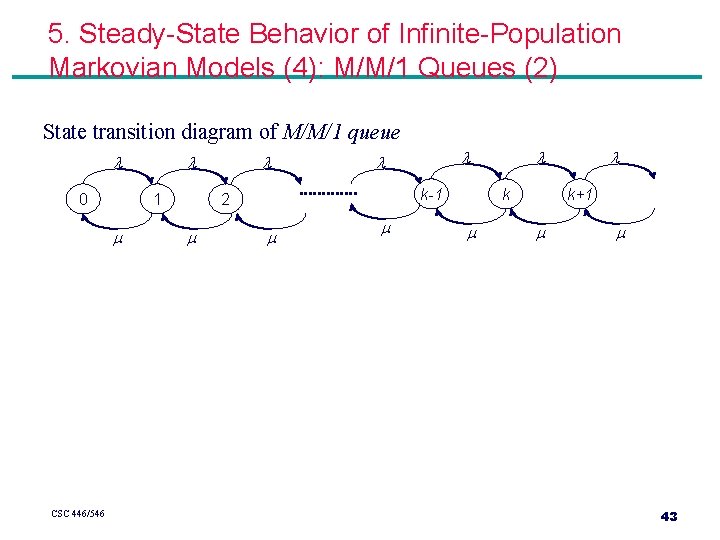
5. Steady-State Behavior of Infinite-Population Markovian Models (4): M/M/1 Queues (2) State transition diagram of M/M/1 queue 0 1 CSC 446/546 k-1 2 k k+1 43

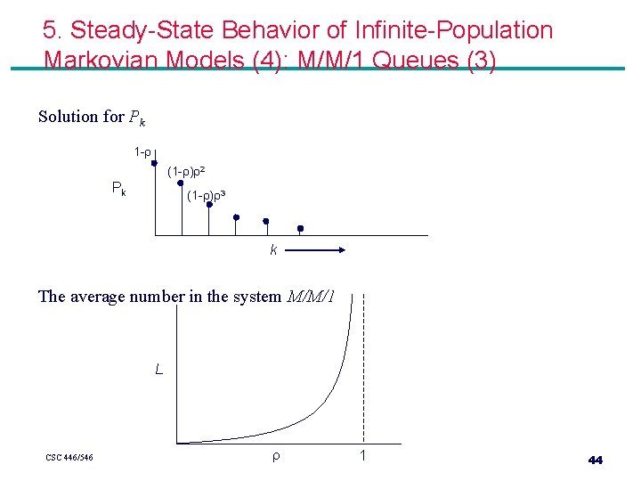
5. Steady-State Behavior of Infinite-Population Markovian Models (4): M/M/1 Queues (3) Solution for Pk 1 - (1 - ) 2 Pk (1 - ) 3 k The average number in the system M/M/1 L CSC 446/546 1 44

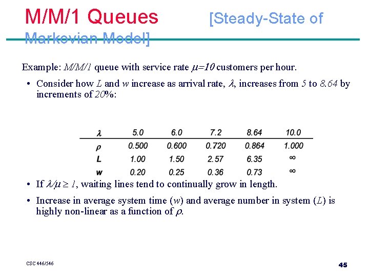
M/M/1 Queues [Steady-State of Markovian Model] Example: M/M/1 queue with service rate =10 customers per hour. • Consider how L and w increase as arrival rate, , increases from 5 to 8. 64 by increments of 20%: • If / ³ 1, waiting lines tend to continually grow in length. • Increase in average system time (w) and average number in system (L) is highly non-linear as a function of . CSC 446/546 45

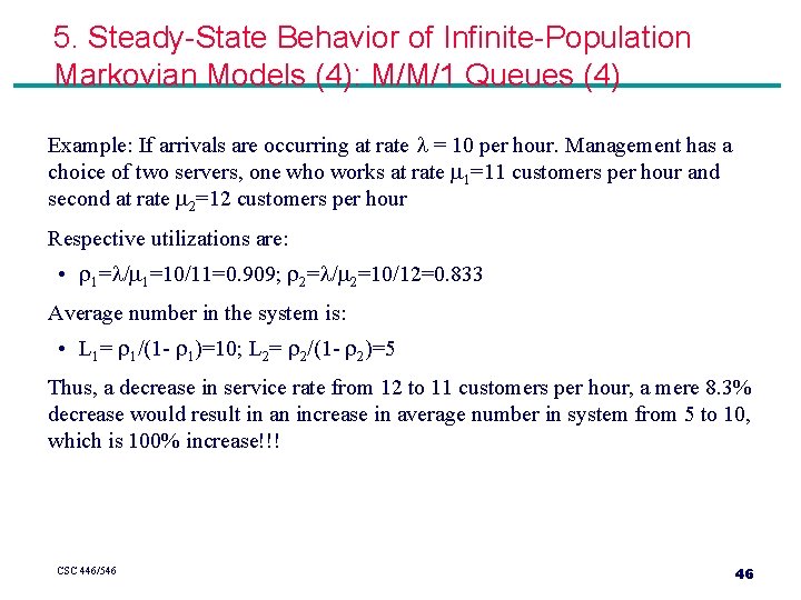
5. Steady-State Behavior of Infinite-Population Markovian Models (4): M/M/1 Queues (4) Example: If arrivals are occurring at rate = 10 per hour. Management has a choice of two servers, one who works at rate 1=11 customers per hour and second at rate 2=12 customers per hour Respective utilizations are: • 1= / 1=10/11=0. 909; 2= / 2=10/12=0. 833 Average number in the system is: • L 1= 1/(1 - 1)=10; L 2= 2/(1 - 2)=5 Thus, a decrease in service rate from 12 to 11 customers per hour, a mere 8. 3% decrease would result in an increase in average number in system from 5 to 10, which is 100% increase!!! CSC 446/546 46

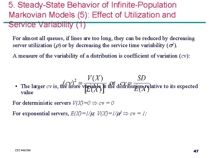
5. Steady-State Behavior of Infinite-Population Markovian Models (5): Effect of Utilization and Service Variability (1) For almost all queues, if lines are too long, they can be reduced by decreasing server utilization ( ) or by decreasing the service time variability (s 2). A measure of the variability of a distribution is coefficient of variation (cv): • The larger cv is, the more variable is the distribution relative to its expected value For deterministic servers V(X)=0 cv = 0 For exponential servers, E(X)=1/ ; V(X)=1/ 2 cv = 1; CSC 446/546 47

5. Steady-State Behavior of Infinite-Population Markovian Models (5): Effect of Utilization and Service Variability (2) Consider LQ for any M/G/1 queue: LQ for M/M/1 queue CSC 446/546 Corrects the M/M/1 formula to account for a non-exponential service time dist’n 48

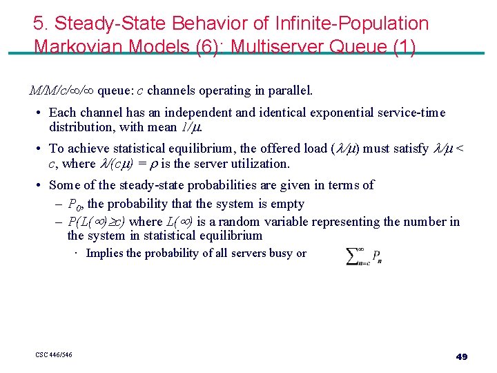
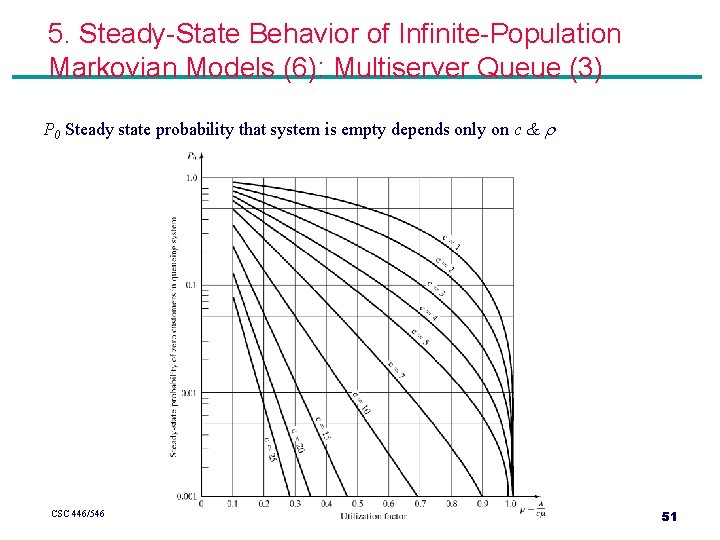
5. Steady-State Behavior of Infinite-Population Markovian Models (6): Multiserver Queue (1) M/M/c/∞/∞ queue: c channels operating in parallel. • Each channel has an independent and identical exponential service-time distribution, with mean 1/. • To achieve statistical equilibrium, the offered load ( / ) must satisfy / < c, where /(c ) = is the server utilization. • Some of the steady-state probabilities are given in terms of – P 0, the probability that the system is empty – P(L( ) c) where L( ) is a random variable representing the number in the system in statistical equilibrium · Implies the probability of all servers busy or CSC 446/546 49

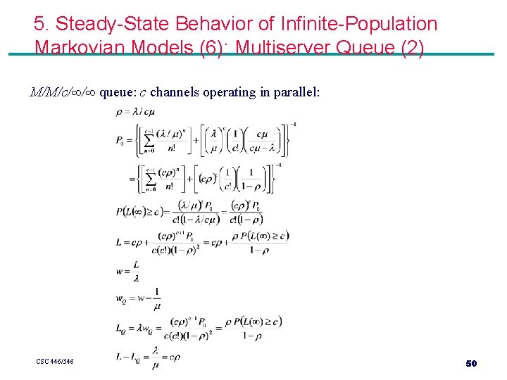
5. Steady-State Behavior of Infinite-Population Markovian Models (6): Multiserver Queue (2) M/M/c/∞/∞ queue: c channels operating in parallel: CSC 446/546 50

5. Steady-State Behavior of Infinite-Population Markovian Models (6): Multiserver Queue (3) P 0 Steady state probability that system is empty depends only on c & CSC 446/546 51

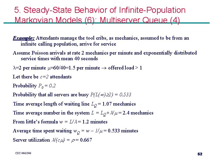
5. Steady-State Behavior of Infinite-Population Markovian Models (6): Multiserver Queue (4) Example: Attendants manage the tool cribs, as mechanics, assumed to be from an infinite calling population, arrive for service Assume Poisson arrivals at rate 2 mechanics per minute and exponentially distributed service times with mean 40 seconds =2 per minute =60/40=1. 5 per minute offered load > 1 Let there be c=2 attendants Probability P 0 = 0. 2 Probability that all servers are busy P(L( ) 2) = 0. 533 Time average length of waiting line LQ = 1. 07 mechanics Time average number in the system L = LQ+ / = 2. 4 mechanics From little’s formula w = L/ = 1. 2 minutes Average time spent waiting w. Q = w – 1/ = 0. 533 minutes Server utilization /(c ) = = 0. 667 CSC 446/546 52

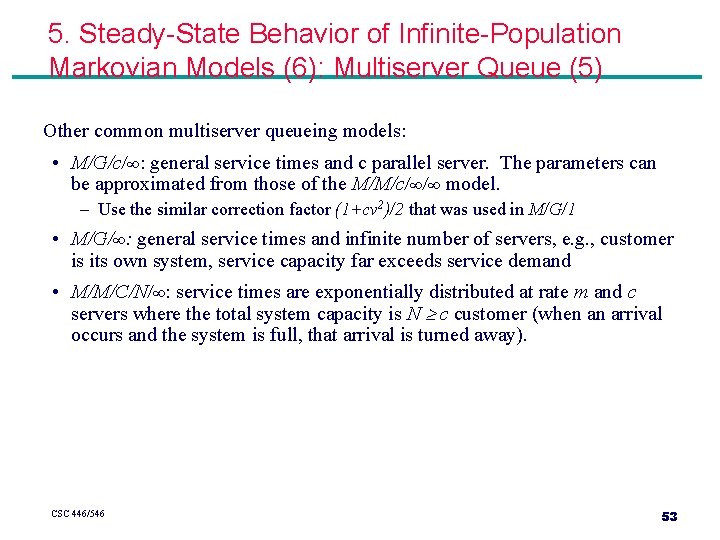
5. Steady-State Behavior of Infinite-Population Markovian Models (6): Multiserver Queue (5) Other common multiserver queueing models: • M/G/c/∞: general service times and c parallel server. The parameters can be approximated from those of the M/M/c/∞/∞ model. – Use the similar correction factor (1+cv 2)/2 that was used in M/G/1 • M/G/∞: general service times and infinite number of servers, e. g. , customer is its own system, service capacity far exceeds service demand • M/M/C/N/∞: service times are exponentially distributed at rate m and c servers where the total system capacity is N c customer (when an arrival occurs and the system is full, that arrival is turned away). CSC 446/546 53

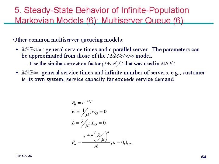
5. Steady-State Behavior of Infinite-Population Markovian Models (6): Multiserver Queue (6) Other common multiserver queueing models: • M/G/c/∞: general service times and c parallel server. The parameters can be approximated from those of the M/M/c/∞/∞ model. – Use the similar correction factor (1+cv 2)/2 that was used in M/G/1 • M/G/∞: general service times and infinite number of servers, e. g. , customer is its own system, service capacity far exceeds service demand CSC 446/546 54

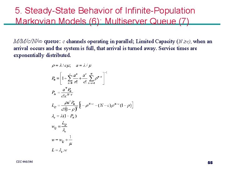
5. Steady-State Behavior of Infinite-Population Markovian Models (6): Multiserver Queue (7) M/M/c/N/∞ queue: c channels operating in parallel; Limited Capacity (N c), when an arrival occurs and the system is full, that arrival is turned away. Service times are exponentially distributed. CSC 446/546 55

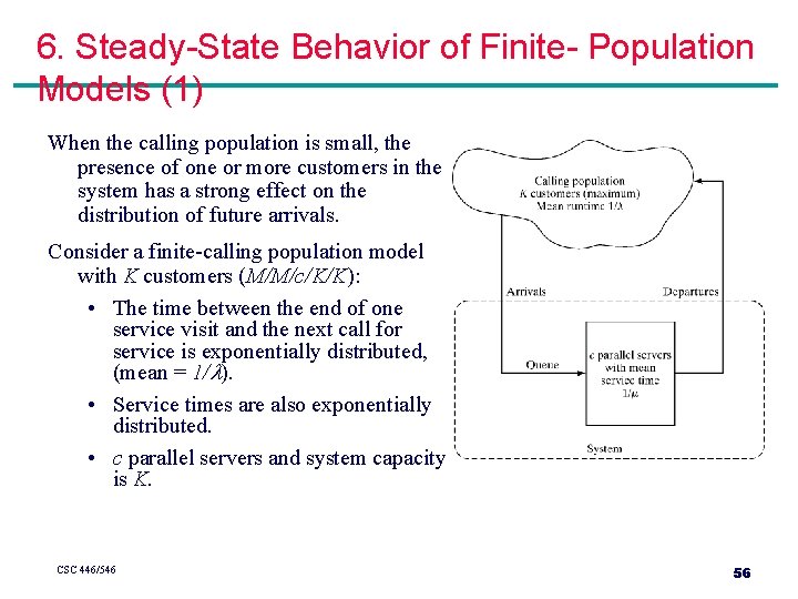
6. Steady-State Behavior of Finite- Population Models (1) When the calling population is small, the presence of one or more customers in the system has a strong effect on the distribution of future arrivals. Consider a finite-calling population model with K customers (M/M/c/K/K): • The time between the end of one service visit and the next call for service is exponentially distributed, (mean = 1/ ). • Service times are also exponentially distributed. • c parallel servers and system capacity is K. CSC 446/546 56

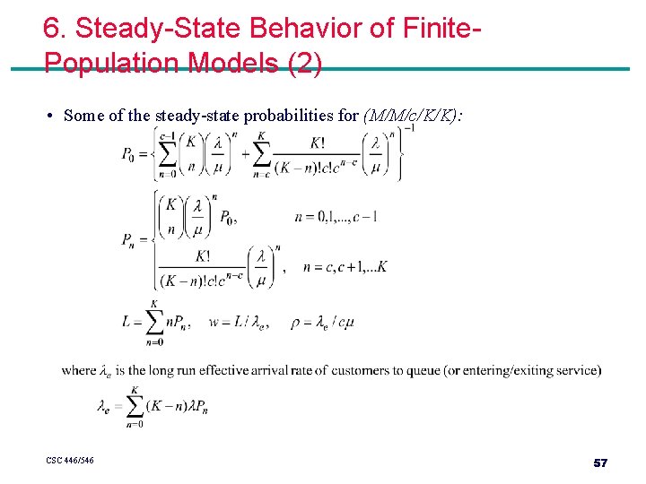
6. Steady-State Behavior of Finite. Population Models (2) • Some of the steady-state probabilities for (M/M/c/K/K): CSC 446/546 57

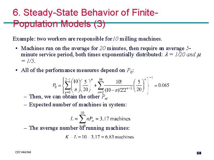
6. Steady-State Behavior of Finite. Population Models (3) Example: two workers are responsible for 10 milling machines. • Machines run on the average for 20 minutes, then require an average 5 minute service period, both times exponentially distributed: = 1/20 and = 1/5. • All of the performance measures depend on P 0: – Then, we can obtain the other Pn. – Expected number of machines in system: – The average number of running machines: CSC 446/546 58

7. Final Summary Introduced basic concepts of queueing models. Show simulation, and some times mathematical analysis, can be used to estimate the performance measures of a system. Commonly used performance measures: L, LQ, w, w. Q, , and e. When simulating any system that evolves over time, analyst must decide whether to study transient behavior or steady-state behavior. • Simple formulas exist for the steady-state behavior of some queues. Simple models can be solved mathematically, and can be useful in providing a rough estimate of a performance measure. CSC 446/546 59