CSC 401 Analysis of Algorithms Chapter 5 3

CSC 401 – Analysis of Algorithms Chapter 5 -- 3 Dynamic Programming Objectives: • • • Present the Dynamic Programming paradigm Review the Matrix Chain-Product problem Discuss the General Technique Solve the 0 -1 Knapsack Problem Introduce pseudo-polynomial-time algorithms CSC 401: Analysis of Algorithms 5 -3 -1

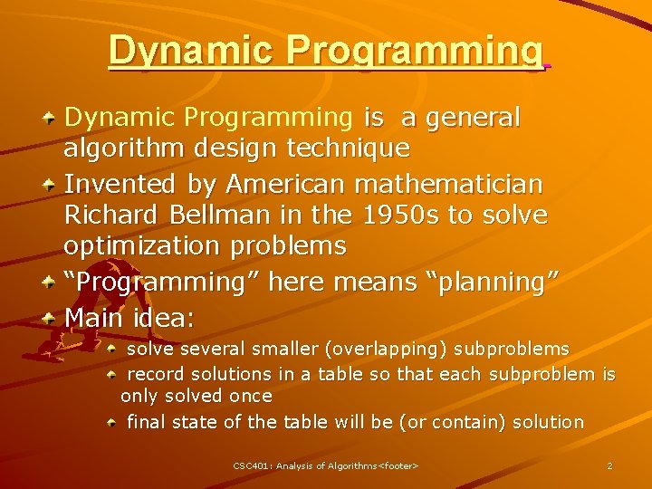
Dynamic Programming is a general algorithm design technique Invented by American mathematician Richard Bellman in the 1950 s to solve optimization problems “Programming” here means “planning” Main idea: solve several smaller (overlapping) subproblems record solutions in a table so that each subproblem is only solved once final state of the table will be (or contain) solution CSC 401: Analysis of Algorithms <footer> 2

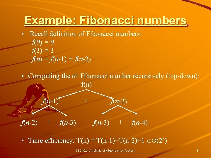
Example: Fibonacci numbers • Recall definition of Fibonacci numbers: f(0) = 0 f(1) = 1 f(n) = f(n-1) + f(n-2) • Computing the nth Fibonacci number recursively (top-down): f(n) f(n-1) + f(n-2) + f(n-3) + f(n-4). . . • Time efficiency: T(n) = T(n-1)+T(n-2)+1 O(2 n) CSC 401: Analysis of Algorithms <footer> 3

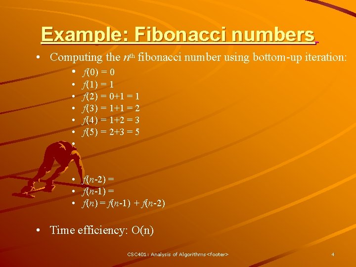
Example: Fibonacci numbers • Computing the nth fibonacci number using bottom-up iteration: • f(0) = 0 • • • f(1) = 1 f(2) = 0+1 = 1 f(3) = 1+1 = 2 f(4) = 1+2 = 3 f(5) = 2+3 = 5 • f(n-2) = • f(n-1) = • f(n) = f(n-1) + f(n-2) • Time efficiency: O(n) CSC 401: Analysis of Algorithms <footer> 4

Examples of Dynamic Programming Algorithms • Computing binomial coefficients • Optimal chain matrix multiplication • Constructing an optimal binary search tree • Warshall’s algorithm for transitive closure • Floyd’s algorithms for all-pairs shortest paths • Some instances of difficult discrete optimization problems: • travelling salesman • knapsack CSC 401: Analysis of Algorithms <footer> 5

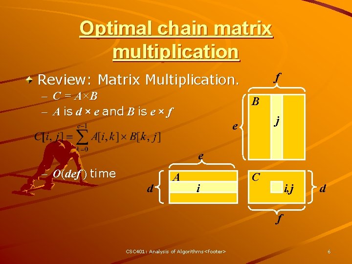
Optimal chain matrix multiplication f Review: Matrix Multiplication. – C = A×B – A is d × e and B is e × f B j e e – O(def ) time d A i C i, j d f CSC 401: Analysis of Algorithms <footer> 6

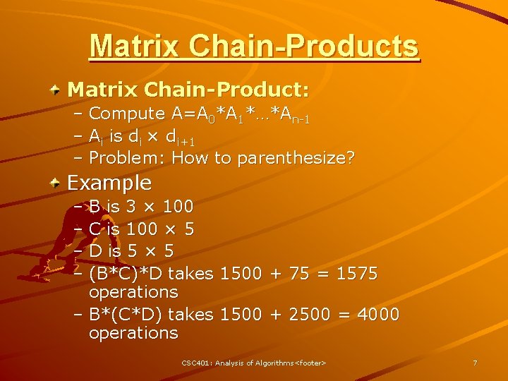
Matrix Chain-Products Matrix Chain-Product: – Compute A=A 0*A 1*…*An-1 – Ai is di × di+1 – Problem: How to parenthesize? Example – B is 3 × 100 – C is 100 × 5 – D is 5 × 5 – (B*C)*D takes 1500 + 75 = 1575 operations – B*(C*D) takes 1500 + 2500 = 4000 operations CSC 401: Analysis of Algorithms <footer> 7

A Brute-force Approach Matrix Chain-Product Algorithm: – Try all possible ways to parenthesize A=A 0*A 1*…*An-1 – Calculate number of operations for each one – Pick the best one Running time: – The number of paranethesizations is equal to the number of binary trees with n nodes – This is exponential! – It is called the Catalan number, and it is almost 4 n. – This is a terrible algorithm! CSC 401: Analysis of Algorithms <footer> 8

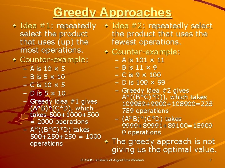
Greedy Approaches Idea #1: repeatedly select the product that uses (up) the most operations. Counter-example: – – – A is 10 × 5 B is 5 × 10 C is 10 × 5 D is 5 × 10 Greedy idea #1 gives (A*B)*(C*D), which takes 500+1000+500 = 2000 operations – A*((B*C)*D) takes 500+250 = 1000 operations Idea #2: repeatedly select the product that uses the fewest operations. Counter-example: – – – A is 101 × 11 B is 11 × 9 C is 9 × 100 D is 100 × 99 Greedy idea #2 gives A*((B*C)*D)), which takes 109989+9900+108900=228 789 operations – (A*B)*(C*D) takes 9999+89991+89100=18909 0 operations The greedy approach is not giving us the optimal value. CSC 401: Analysis of Algorithms <footer> 9

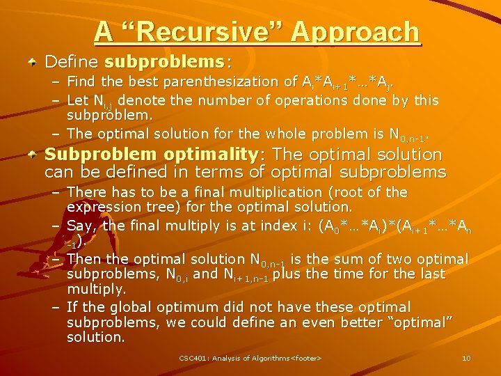
A “Recursive” Approach Define subproblems: – Find the best parenthesization of Ai*Ai+1*…*Aj. – Let Ni, j denote the number of operations done by this subproblem. – The optimal solution for the whole problem is N 0, n-1. Subproblem optimality: The optimal solution can be defined in terms of optimal subproblems – There has to be a final multiplication (root of the expression tree) for the optimal solution. – Say, the final multiply is at index i: (A 0*…*Ai)*(Ai+1*…*An -1). – Then the optimal solution N 0, n-1 is the sum of two optimal subproblems, N 0, i and Ni+1, n-1 plus the time for the last multiply. – If the global optimum did not have these optimal subproblems, we could define an even better “optimal” solution. CSC 401: Analysis of Algorithms <footer> 10

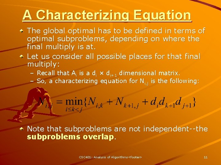
A Characterizing Equation The global optimal has to be defined in terms of optimal subproblems, depending on where the final multiply is at. Let us consider all possible places for that final multiply: – Recall that Ai is a di × di+1 dimensional matrix. – So, a characterizing equation for Ni, j is the following: Note that subproblems are not independent--the subproblems overlap. CSC 401: Analysis of Algorithms <footer> 11

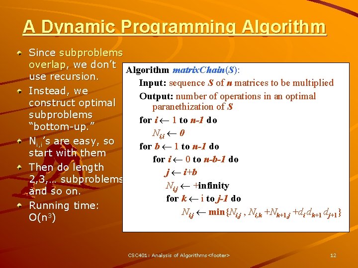
A Dynamic Programming Algorithm Since subproblems overlap, we don’t Algorithm matrix. Chain(S): use recursion. Input: sequence S of n matrices to be multiplied Instead, we Output: number of operations in an optimal construct optimal paranethization of S subproblems for i 1 to n-1 do “bottom-up. ” Ni, i 0 Ni, i’s are easy, so for b 1 to n-1 do start with them for i 0 to n-b-1 do Then do length j i+b 2, 3, … subproblems, Ni, j +infinity and so on. for k i to j-1 do Running time: Ni, j min{Ni, j , Ni, k +Nk+1, j +di dk+1 dj+1} O(n 3) CSC 401: Analysis of Algorithms <footer> 12

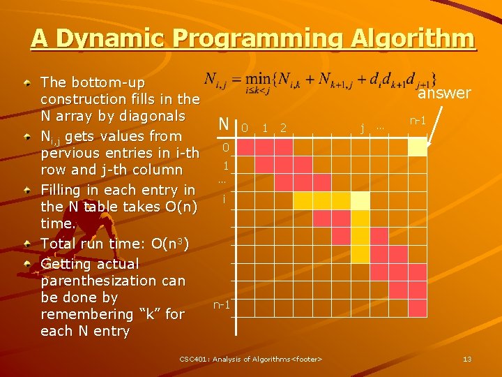
A Dynamic Programming Algorithm The bottom-up construction fills in the N array by diagonals Ni, j gets values from pervious entries in i-th row and j-th column Filling in each entry in the N table takes O(n) time. Total run time: O(n 3) Getting actual parenthesization can be done by remembering “k” for each N entry answer N 0 1 2 j … n-1 0 1 … i n-1 CSC 401: Analysis of Algorithms <footer> 13

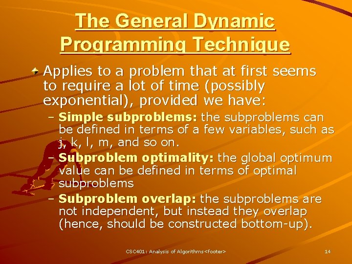
The General Dynamic Programming Technique Applies to a problem that at first seems to require a lot of time (possibly exponential), provided we have: – Simple subproblems: the subproblems can be defined in terms of a few variables, such as j, k, l, m, and so on. – Subproblem optimality: the global optimum value can be defined in terms of optimal subproblems – Subproblem overlap: the subproblems are not independent, but instead they overlap (hence, should be constructed bottom-up). CSC 401: Analysis of Algorithms <footer> 14

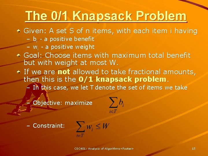
The 0/1 Knapsack Problem Given: A set S of n items, with each item i having – bi - a positive benefit – wi - a positive weight Goal: Choose items with maximum total benefit but with weight at most W. If we are not allowed to take fractional amounts, then this is the 0/1 knapsack problem. – In this case, we let T denote the set of items we take – Objective: maximize – Constraint: CSC 401: Analysis of Algorithms <footer> 15

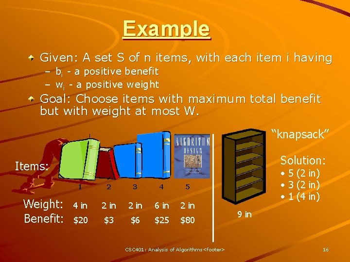
Example Given: A set S of n items, with each item i having – bi - a positive benefit – wi - a positive weight Goal: Choose items with maximum total benefit but with weight at most W. “knapsack” Solution: Items: Weight: Benefit: 1 2 3 4 5 4 in 2 in 6 in 2 in $20 $3 $6 $25 $80 CSC 401: Analysis of Algorithms <footer> • 5 (2 in) • 3 (2 in) • 1 (4 in) 9 in 16

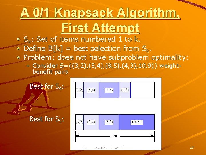
A 0/1 Knapsack Algorithm, First Attempt Sk: Set of items numbered 1 to k. Define B[k] = best selection from Sk. Problem: does not have subproblem optimality: – Consider S={(3, 2), (5, 4), (8, 5), (4, 3), 10, 9)} weightbenefit pairs Best for S 4: Best for S 5: CSC 401: Analysis of Algorithms <footer> 17

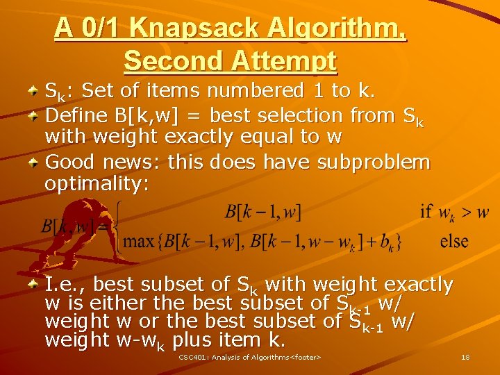
A 0/1 Knapsack Algorithm, Second Attempt Sk: Set of items numbered 1 to k. Define B[k, w] = best selection from Sk with weight exactly equal to w Good news: this does have subproblem optimality: I. e. , best subset of Sk with weight exactly w is either the best subset of Sk-1 w/ weight w or the best subset of Sk-1 w/ weight w-wk plus item k. CSC 401: Analysis of Algorithms <footer> 18

The 0/1 Knapsack Algorithm Recall definition of B[k, w]: Since B[k, w] is defined in terms of B[k-1, *], we can reuse the same array Running time: O(n. W). Not a polynomial-time algorithm if W is large This is a pseudopolynomial time algorithm Algorithm 01 Knapsack(S, W): Input: set S of items w/ benefit bi and weight wi; max. weight W Output: benefit of best subset with weight at most W for w 0 to W do B[w] 0 for k 1 to n do for w W downto wk do if B[w-wk]+bk > B[w] then B[w] B[w-wk]+bk CSC 401: Analysis of Algorithms <footer> 19

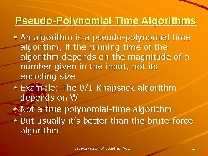
Pseudo-Polynomial Time Algorithms An algorithm is a pseudo-polynomial time algorithm, if the running time of the algorithm depends on the magnitude of a number given in the input, not its encoding size Example: The 0/1 Knapsack algorithm depends on W Not a true polynomial-time algorithm But usually it’s better than the brute-force algorithm CSC 401: Analysis of Algorithms <footer> 20