Optimization Methods in Energy and Power Systems Lecture

Optimization Methods in Energy and Power Systems Lecture 4: Sensitivity Analysis & LP Duality Mahdi Pourakbari Kasmaei, 2019 Thursday, 21 March 2019

LP Problems (Sensitivity Analysis & LP Duality) ü Marginal Values (Shadow Prices and Reduced Costs) and Sensitivity Ranges are used in conducting Sensitivity Analysis. ü Simplex method (used in solvers) provide extra information than the optimal solution. It provides Marginal Values. 2

LP Problems (Sensitivity Analysis) ü Marginal values give information on the variability of the Optimal Solution due to changes in the Input Data. ü Shadow Prices are associated with the right-hand side (RHS) of the constraints. ü Reduced Costs are associated with the basic variables and their corresponding bounds. 3

LP Problems (Sensitivity Analysis) Only use the Concepts of Marginal Values for LP Problems. 4

LP Problems (Shadow Prices) ü One unit change in the RHS of the constraints results in a change in the Objective Function. • Positive Shadow Price means that the objective function will increase by increasing the RHS by one unit. • Negative Shadow Price means the objective function will decrease by increasing the RHS by one unit. 5

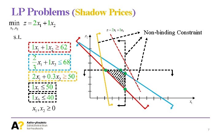
LP Problems (Shadow Prices) ü If there exist non-binding constraints in the LP problem, changing the RHS results in no change in the Objective Function. The Shadow Price is Zero. • Binding Constraints!? ? Those constraint that restrict the optimal solution; Intersected Lines. • Non-Binding Constraints!? ? Those constraint that are not affecting the Optimal Solution. 6

LP Problems (Shadow Prices) Non-binding Constraint 7

LP Problems (Shadow Prices) Binding or Non-Binding Constraints Could become Non-Binding or Binding ones as data Change. 8

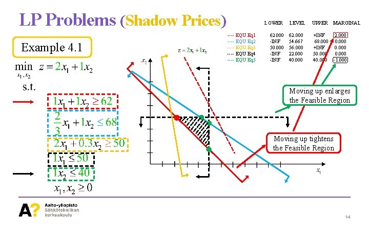
LP Problems (Shadow Prices) ü How we can take the advantage of Shadow Prices? ! • To objective function is improved by weakening (relaxing) the binding constraint, i. e. , enlarging the feasible region. • Improving for Minimization and Maximization problems mean decreases and increases the RHS, respectively. 9

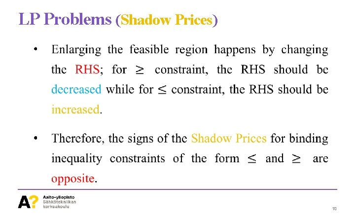
LP Problems (Shadow Prices) 10

LP Problems (Shadow Prices) • As discussed, any Equality Constraint can be transformed into two inequality constraints; in this case, at most one of them will have a nonzero Shadow Price. 11

Solving LP Problems (Shadow Prices) ü Sign of the Shadow Price can be used to infer the sign of the binding constraint: • Considering a Minimization Problem, if the Shadow Price of a binding Equality Constraint is Negative, it means that the Objective Function will decrease (improve) if the RHS increases. 12

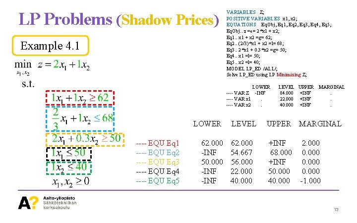
LP Problems (Shadow Prices) Example 4. 1 VARIABLES Z; POSITIVE VARIABLES x 1, x 2; EQUATIONS Eq. Obj, Eq 1, Eq 2, Eq 3, Eq 4, Eq 5; Eq. Obj. . z =e= 2*x 1 + x 2; Eq 1. . x 1 + x 2 =g= 62; Eq 2. . (2/3)*x 1 + x 2 =l= 68; Eq 3. . 2*x 1 + 0. 3*x 2 =g= 50; Eq 4. . x 1 =l= 50; Eq 5. . x 2 =l= 40; MODEL LP_ED /ALL/; Solve LP_ED using LP Minimizing Z; LOWER ---- VAR Z -INF ---- VAR x 1. ---- VAR x 2. LOWER ---- EQU Eq 1 ---- EQU Eq 2 ---- EQU Eq 3 ---- EQU Eq 4 ---- EQU Eq 5 LEVEL 62. 000 -INF 54. 667 50. 000 56. 000 -INF 22. 000 -INF 40. 000 LEVEL UPPER 84. 000 +INF 22. 000 +INF 40. 000 +INF MARGINAL. . . UPPER MARGINAL +INF 68. 000 +INF 50. 000 40. 000 2. 000 0. 000 -1. 000 13

LP Problems (Shadow Prices) Example 4. 1 LOWER ---- EQU Eq 1 ---- EQU Eq 2 ---- EQU Eq 3 ---- EQU Eq 4 ---- EQU Eq 5 LEVEL 62. 000 -INF 54. 667 50. 000 56. 000 -INF 22. 000 -INF 40. 000 UPPER MARGINAL +INF 68. 000 +INF 50. 000 40. 000 2. 000 0. 000 -1. 000 Moving up enlarges the Feasible Region Moving up tightens the Feasible Region 14

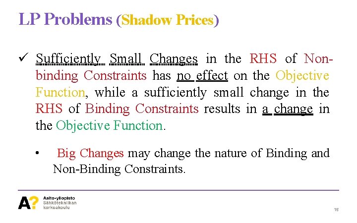
LP Problems (Shadow Prices) ü Sufficiently Small Changes in the RHS of Nonbinding Constraints has no effect on the Objective Function, while a sufficiently small change in the RHS of Binding Constraints results in a change in the Objective Function. • Big Changes may change the nature of Binding and Non-Binding Constraints. 15

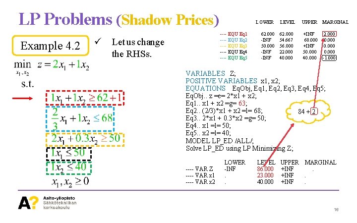
LP Problems (Shadow Prices) Example 4. 2 LOWER ---- EQU Eq 1 ---- EQU Eq 2 ---- EQU Eq 3 ---- EQU Eq 4 ---- EQU Eq 5 ü Let us change the RHSs. LEVEL 62. 000 -INF 54. 667 50. 000 56. 000 -INF 22. 000 -INF 40. 000 UPPER MARGINAL +INF 68. 000 +INF 50. 000 40. 000 2. 000 0. 000 -1. 000 VARIABLES Z; POSITIVE VARIABLES x 1, x 2; EQUATIONS Eq. Obj, Eq 1, Eq 2, Eq 3, Eq 4, Eq 5; Eq. Obj. . z =e= 2*x 1 + x 2; Eq 1. . x 1 + x 2 =g= 63; Eq 2. . (2/3)*x 1 + x 2 =l= 68; 84 + 2 Eq 3. . 2*x 1 + 0. 3*x 2 =g= 50; Eq 4. . x 1 =l= 50; Eq 5. . x 2 =l= 40; MODEL LP_ED /ALL/; Solve LP_ED using LP Minimizing Z; ---- VAR Z ---- VAR x 1 ---- VAR x 2 LOWER -INF. . LEVEL 86. 000 23. 000 40. 000 UPPER MARGINAL +INF. 16

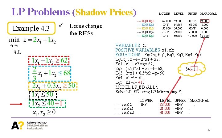
LP Problems (Shadow Prices) Example 4. 3 LOWER ---- EQU Eq 1 ---- EQU Eq 2 ---- EQU Eq 3 ---- EQU Eq 4 ---- EQU Eq 5 ü Let us change the RHSs. LEVEL 62. 000 -INF 54. 667 50. 000 56. 000 -INF 22. 000 -INF 40. 000 UPPER MARGINAL +INF 68. 000 +INF 50. 000 40. 000 2. 000 0. 000 -1. 000 VARIABLES Z; POSITIVE VARIABLES x 1, x 2; EQUATIONS Eq. Obj, Eq 1, Eq 2, Eq 3, Eq 4, Eq 5; Eq. Obj. . z =e= 2*x 1 + x 2; Eq 1. . x 1 + x 2 =g= 62; Eq 2. . (2/3)*x 1 + x 2 =l= 68; 84 - 1 Eq 3. . 2*x 1 + 0. 3*x 2 =g= 50; Eq 4. . x 1 =l= 50; Eq 5. . x 2 =l= 41; MODEL LP_ED /ALL/; Solve LP_ED using LP Minimizing Z; ---- VAR Z ---- VAR x 1 ---- VAR x 2 LOWER -INF. . LEVEL 83. 000 21. 000 41. 000 UPPER MARGINAL +INF. 17

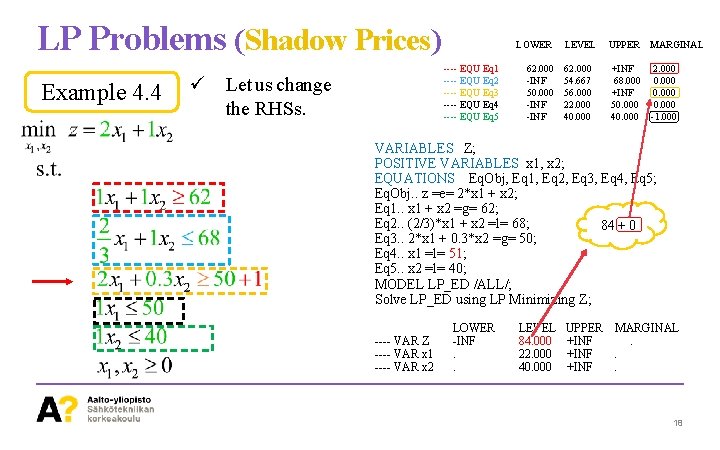
LP Problems (Shadow Prices) Example 4. 4 LOWER ---- EQU Eq 1 ---- EQU Eq 2 ---- EQU Eq 3 ---- EQU Eq 4 ---- EQU Eq 5 ü Let us change the RHSs. LEVEL 62. 000 -INF 54. 667 50. 000 56. 000 -INF 22. 000 -INF 40. 000 UPPER MARGINAL +INF 68. 000 +INF 50. 000 40. 000 2. 000 0. 000 -1. 000 VARIABLES Z; POSITIVE VARIABLES x 1, x 2; EQUATIONS Eq. Obj, Eq 1, Eq 2, Eq 3, Eq 4, Eq 5; Eq. Obj. . z =e= 2*x 1 + x 2; Eq 1. . x 1 + x 2 =g= 62; Eq 2. . (2/3)*x 1 + x 2 =l= 68; 84 + 0 Eq 3. . 2*x 1 + 0. 3*x 2 =g= 50; Eq 4. . x 1 =l= 51; Eq 5. . x 2 =l= 40; MODEL LP_ED /ALL/; Solve LP_ED using LP Minimizing Z; ---- VAR Z ---- VAR x 1 ---- VAR x 2 LOWER -INF. . LEVEL 84. 000 22. 000 40. 000 UPPER MARGINAL +INF. 18

LP Problems (Reduced Costs) ü The Marginal Value corresponds to a decision variable is interpreted as its Reduced Cost. ü Reduced Cost stand for the rate of change of the Objective Function for one unit increase in the Bound of a Variable. 19

LP Problems (Reduced Costs) ü If a non-basic variable has a Positive Reduced Cost, the Objective Function will increase with a one unit increase in the binding bound, while if a non-basic variable has a Negative Reduced Cost, the Objective Function will decrease. ü The Reduced Cost of a basic variable is Zero if its bounds are nonbinding and therefore do not constrain the optimal solution. 20

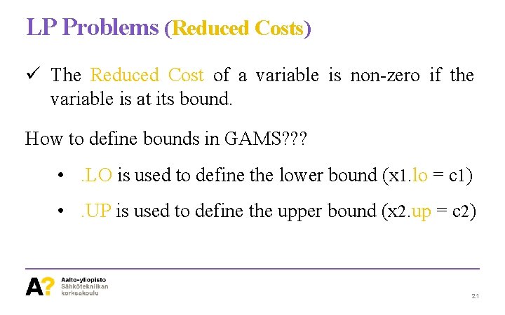
LP Problems (Reduced Costs) ü The Reduced Cost of a variable is non-zero if the variable is at its bound. How to define bounds in GAMS? ? ? • . LO is used to define the lower bound (x 1. lo = c 1) • . UP is used to define the upper bound (x 2. up = c 2) 21

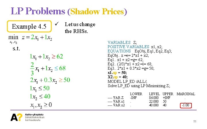
LP Problems (Shadow Prices) Example 4. 5 ü Let us change the RHSs. VARIABLES Z; POSITIVE VARIABLES x 1, x 2; EQUATIONS Eq. Obj, Eq 1, Eq 2, Eq 3; Eq. Obj. . z =e= 2*x 1 + x 2; Eq 1. . x 1 + x 2 =g= 62; Eq 2. . (2/3)*x 1 + x 2 =l= 68; Eq 3. . 2*x 1 + 0. 3*x 2 =g= 50; x 1. up = 50; X 2. up = 40; MODEL LP_ED /ALL/; Solve LP_ED using LP Minimizing Z; ---- VAR Z ---- VAR x 1 ---- VAR x 2 LOWER -INF. . LEVEL 84. 000 22. 000 40. 000 UPPER +INF 50 40 MARGINAL. . -1. 00 22

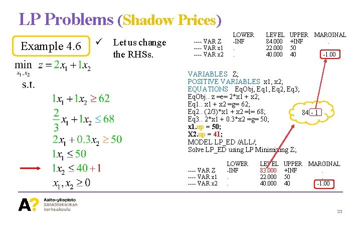
LP Problems (Shadow Prices) Example 4. 6 ü Let us change the RHSs. ---- VAR Z ---- VAR x 1 ---- VAR x 2 LOWER -INF. . LEVEL 84. 000 22. 000 40. 000 UPPER +INF 50 40 MARGINAL. . -1. 00 VARIABLES Z; POSITIVE VARIABLES x 1, x 2; EQUATIONS Eq. Obj, Eq 1, Eq 2, Eq 3; Eq. Obj. . z =e= 2*x 1 + x 2; Eq 1. . x 1 + x 2 =g= 62; Eq 2. . (2/3)*x 1 + x 2 =l= 68; 84 - 1 Eq 3. . 2*x 1 + 0. 3*x 2 =g= 50; x 1. up = 50; X 2. up = 41; MODEL LP_ED /ALL/; Solve LP_ED using LP Minimizing Z; ---- VAR Z ---- VAR x 1 ---- VAR x 2 LOWER -INF. . LEVEL 83. 000 22. 000 40. 000 UPPER +INF 50 40 MARGINAL. . -1. 00 23

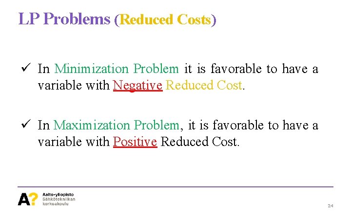
LP Problems (Reduced Costs) ü In Minimization Problem it is favorable to have a variable with Negative Reduced Cost. ü In Maximization Problem, it is favorable to have a variable with Positive Reduced Cost. 24

LP Problems (Sensitivity Analysis) Analysis based on Marginal Values are only Valid for Small Changes. 25

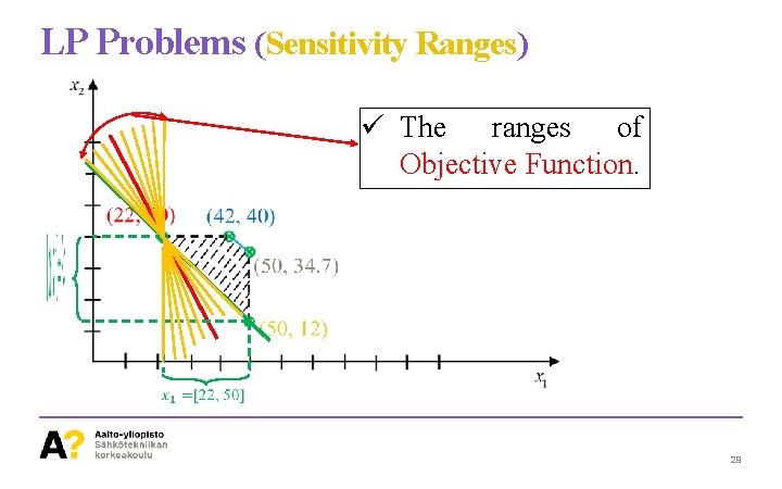
LP Problems (Sensitivity Ranges) ü Sensitivity Ranges Function Value. with constant Objective • Ranges of Decision Variables under this condition depends on the Objective Function. • It can be a unique Optimal Point, or it can be a range of variables corresponding to the Optimal Solution. 26

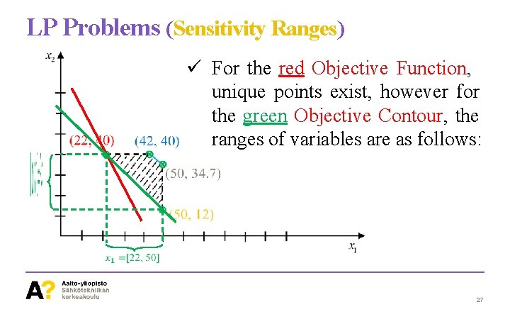
LP Problems (Sensitivity Ranges) ü For the red Objective Function, unique points exist, however for the green Objective Contour, the ranges of variables are as follows: 27

LP Problems (Sensitivity Ranges) ü Sensitivity ranges with Constant Basis. • Ranges of the Objective Function is determined by changing the slope of Objective Function until the Optimal Solution Changes (It converges to another Extreme Point) 28

LP Problems (Sensitivity Ranges) ü The ranges of Objective Function. 29

LP Problems Duality 30

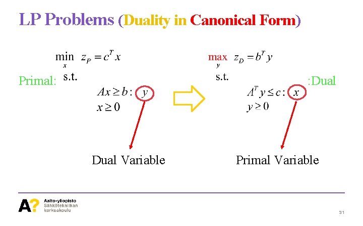
LP Problems (Duality in Canonical Form) Primal: : Dual Variable Primal Variable 31

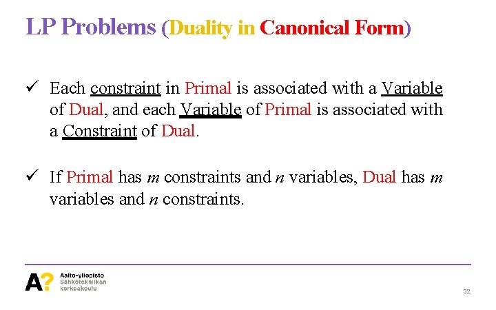
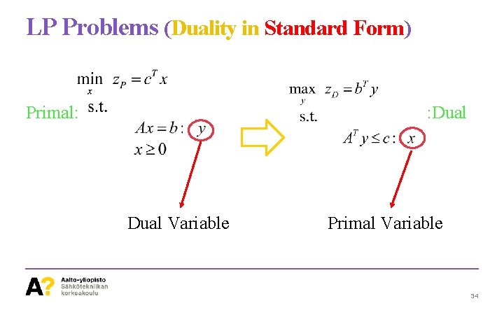
LP Problems (Duality in Canonical Form) ü Each constraint in Primal is associated with a Variable of Dual, and each Variable of Primal is associated with a Constraint of Dual. ü If Primal has m constraints and n variables, Dual has m variables and n constraints. 32

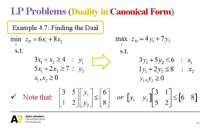
LP Problems (Duality in Canonical Form) Example 4. 7: Finding the Dual ü Note that: 33

LP Problems (Duality in Standard Form) Primal: : Dual Variable Primal Variable 34

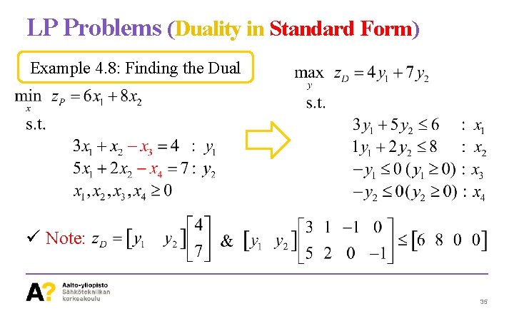
LP Problems (Duality in Standard Form) Example 4. 8: Finding the Dual ü Note: 35

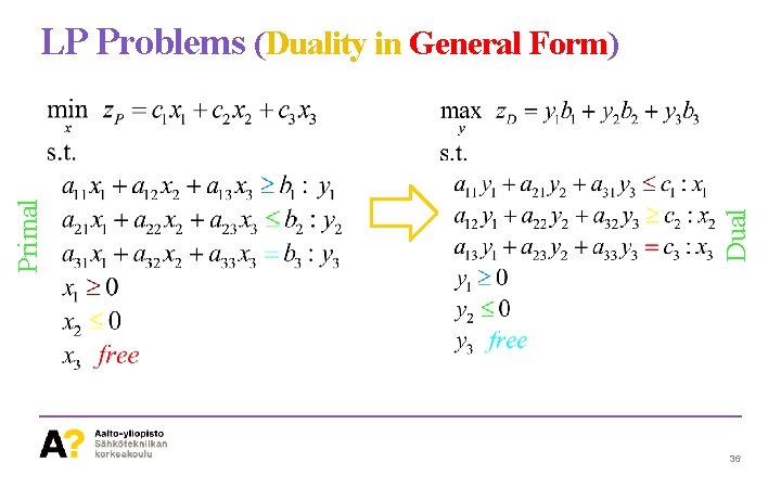
Dual Primal LP Problems (Duality in General Form) 36

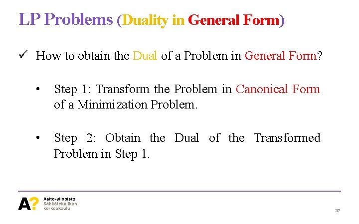
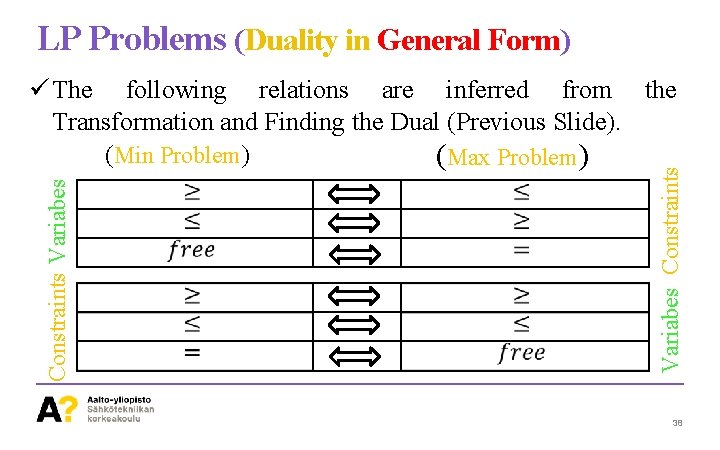
LP Problems (Duality in General Form) ü How to obtain the Dual of a Problem in General Form? • Step 1: Transform the Problem in Canonical Form of a Minimization Problem. • Step 2: Obtain the Dual of the Transformed Problem in Step 1. 37

LP Problems (Duality in General Form) Variabes Constraints Variabes ü The following relations are inferred from the Transformation and Finding the Dual (Previous Slide). (Min Problem) (Max Problem) 38

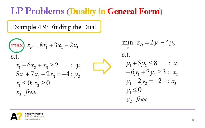
LP Problems (Duality in General Form) Example 4. 9: Finding the Dual 39

Thanks! 40