Chapter 7 Optimization Methods Introduction Examples of optimization

Chapter 7 Optimization Methods

Introduction • Examples of optimization problems – IC design (placement, wiring) – Graph theoretic problems (partitioning, coloring, vertex covering) – Planning – Scheduling – Other combinatorial optimization problems (knapsack, TSP) • Approaches – – AI: state space search NN Genetic algorithms Mathematical programming

Introduction • NN models to cover – Continuous Hopfield mode • Combinatorial optimization – Simulated annealing • Escape from local minimum – Boltzmann machine (§ 6. 4) – Evolutionary computing (genetic algorithms)

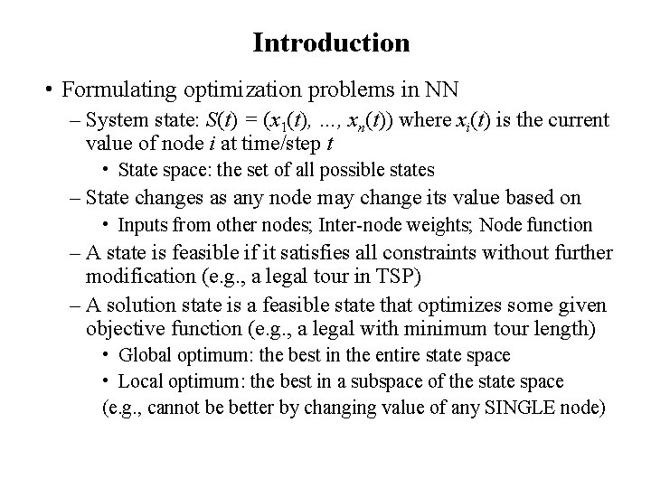
Introduction • Formulating optimization problems in NN – System state: S(t) = (x 1(t), …, xn(t)) where xi(t) is the current value of node i at time/step t • State space: the set of all possible states – State changes as any node may change its value based on • Inputs from other nodes; Inter-node weights; Node function – A state is feasible if it satisfies all constraints without further modification (e. g. , a legal tour in TSP) – A solution state is a feasible state that optimizes some given objective function (e. g. , a legal with minimum tour length) • Global optimum: the best in the entire state space • Local optimum: the best in a subspace of the state space (e. g. , cannot be better by changing value of any SINGLE node)

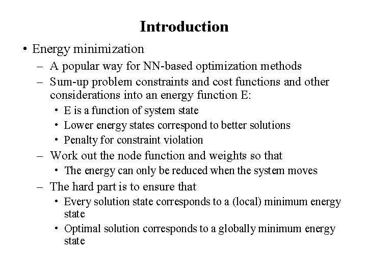
Introduction • Energy minimization – A popular way for NN-based optimization methods – Sum-up problem constraints and cost functions and other considerations into an energy function E: • E is a function of system state • Lower energy states correspond to better solutions • Penalty for constraint violation – Work out the node function and weights so that • The energy can only be reduced when the system moves – The hard part is to ensure that • Every solution state corresponds to a (local) minimum energy state • Optimal solution corresponds to a globally minimum energy state

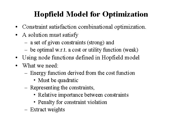
Hopfield Model for Optimization • Constraint satisfaction combinational optimization. • A solution must satisfy – a set of given constraints (strong) and – be optimal w. r. t. a cost or utility function (weak) • Using node functions defined in Hopfield model • What we need: – Energy function derived from the cost function • Must be quadratic – Representing the constraints, • Relative importance between constraints • Penalty for constraint violation – Extract weights

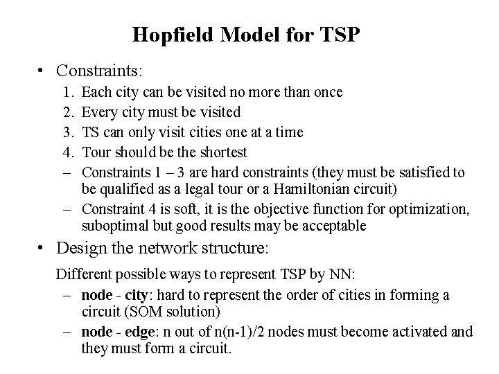
Hopfield Model for TSP • Constraints: 1. 2. 3. 4. – Each city can be visited no more than once Every city must be visited TS can only visit cities one at a time Tour should be the shortest Constraints 1 – 3 are hard constraints (they must be satisfied to be qualified as a legal tour or a Hamiltonian circuit) – Constraint 4 is soft, it is the objective function for optimization, suboptimal but good results may be acceptable • Design the network structure: Different possible ways to represent TSP by NN: – node - city: hard to represent the order of cities in forming a circuit (SOM solution) – node - edge: n out of n(n-1)/2 nodes must become activated and they must form a circuit.

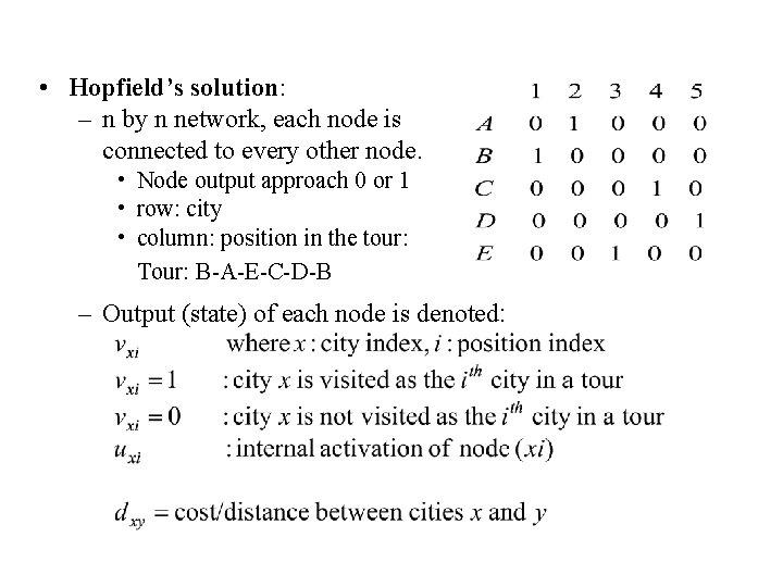
• Hopfield’s solution: – n by n network, each node is connected to every other node. • Node output approach 0 or 1 • row: city • column: position in the tour: Tour: B-A-E-C-D-B – Output (state) of each node is denoted:

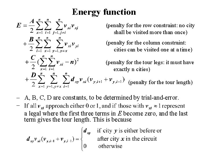
Energy function (penalty for the row constraint: no city shall be visited more than once) (penalty for the column constraint: cities can be visited one at a time) (penalty for the tour legs: it must have exactly n cities) (penalty for the tour length) – A, B, C, D are constants, to be determined by trial-and-error. – a legal where the first three terms in E become zero, and the last term gives the tour length. This is because

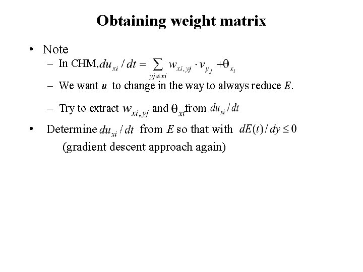
Obtaining weight matrix • Note – In CHM, – We want u to change in the way to always reduce E. – Try to extract • Determine and from E so that with (gradient descent approach again)

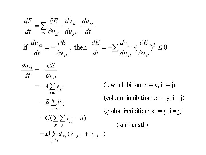
(row inhibition: x = y, i != j) (column inhibition: x != y, i = j) (global inhibition: x != y, i = j) (tour length)

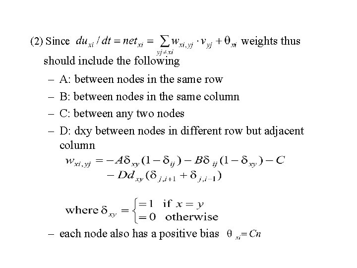
(2) Since , weights thus should include the following – – A: between nodes in the same row B: between nodes in the same column C: between any two nodes D: dxy between nodes in different row but adjacent column – each node also has a positive bias

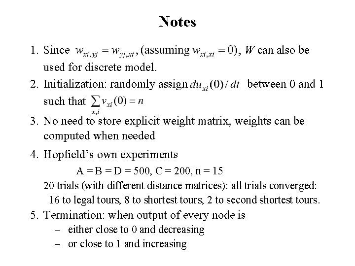
Notes 1. Since used for discrete model. 2. Initialization: randomly assign such that , W can also be between 0 and 1 3. No need to store explicit weight matrix, weights can be computed when needed 4. Hopfield’s own experiments A = B = D = 500, C = 200, n = 15 20 trials (with different distance matrices): all trials converged: 16 to legal tours, 8 to shortest tours, 2 to second shortest tours. 5. Termination: when output of every node is – either close to 0 and decreasing – or close to 1 and increasing

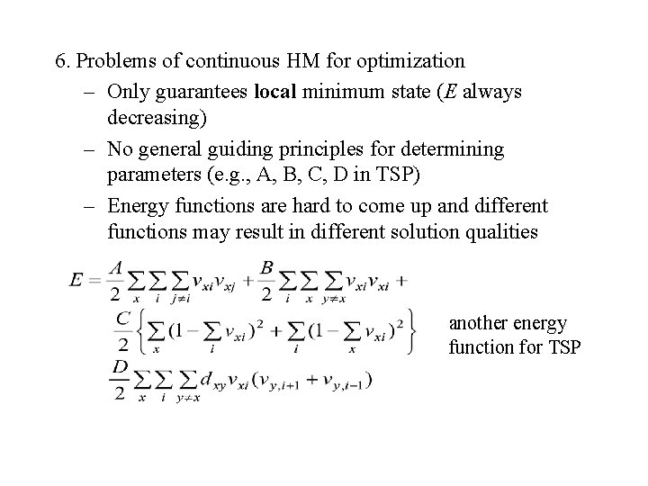
6. Problems of continuous HM for optimization – Only guarantees local minimum state (E always decreasing) – No general guiding principles for determining parameters (e. g. , A, B, C, D in TSP) – Energy functions are hard to come up and different functions may result in different solution qualities another energy function for TSP

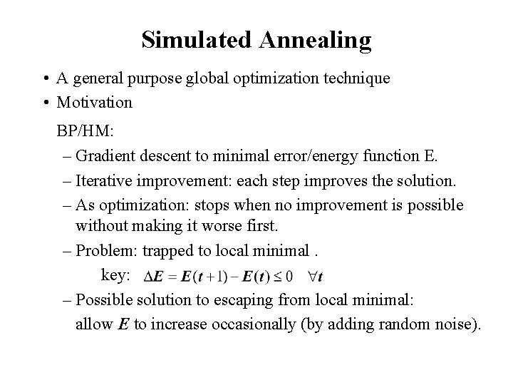
Simulated Annealing • A general purpose global optimization technique • Motivation BP/HM: – Gradient descent to minimal error/energy function E. – Iterative improvement: each step improves the solution. – As optimization: stops when no improvement is possible without making it worse first. – Problem: trapped to local minimal. key: – Possible solution to escaping from local minimal: allow E to increase occasionally (by adding random noise).

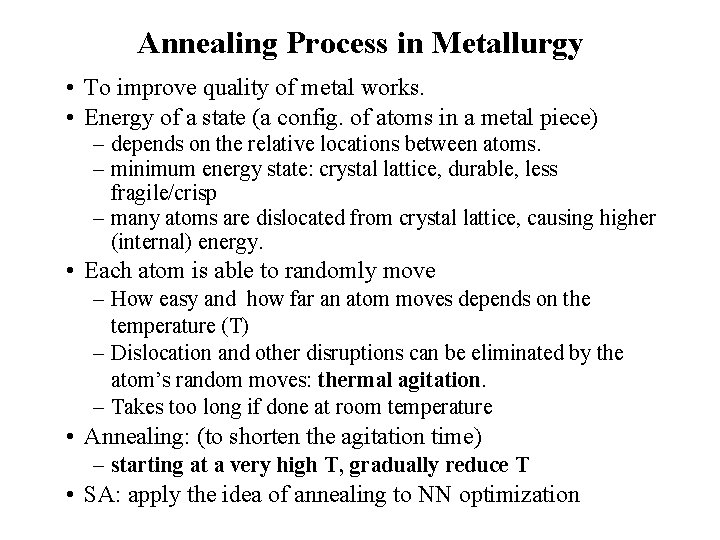
Annealing Process in Metallurgy • To improve quality of metal works. • Energy of a state (a config. of atoms in a metal piece) – depends on the relative locations between atoms. – minimum energy state: crystal lattice, durable, less fragile/crisp – many atoms are dislocated from crystal lattice, causing higher (internal) energy. • Each atom is able to randomly move – How easy and how far an atom moves depends on the temperature (T) – Dislocation and other disruptions can be eliminated by the atom’s random moves: thermal agitation. – Takes too long if done at room temperature • Annealing: (to shorten the agitation time) – starting at a very high T, gradually reduce T • SA: apply the idea of annealing to NN optimization

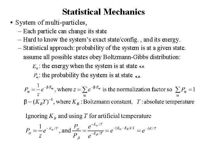
Statistical Mechanics • System of multi-particles, – Each particle can change its state – Hard to know the system’s exact state/config. , and its energy. – Statistical approach: probability of the system is at a given state. assume all possible states obey Boltzmann-Gibbs distribution: : the energy when the system is at state : the probability the system is at state

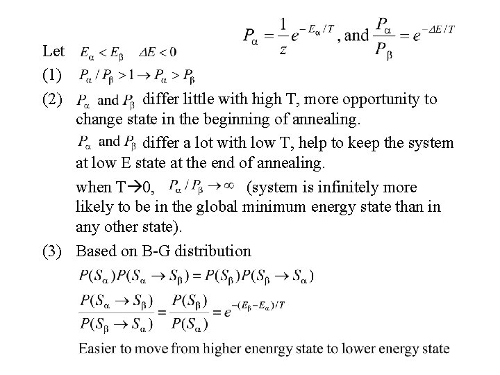
Let (1) (2) differ little with high T, more opportunity to change state in the beginning of annealing. differ a lot with low T, help to keep the system at low E state at the end of annealing. when T 0, (system is infinitely more likely to be in the global minimum energy state than in any other state). (3) Based on B-G distribution

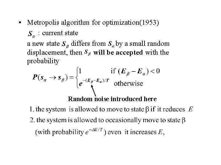
• Metropolis algorithm for optimization(1953) : current state a new state differs from by a small random displacement, then will be accepted with the probability Random noise introduced here

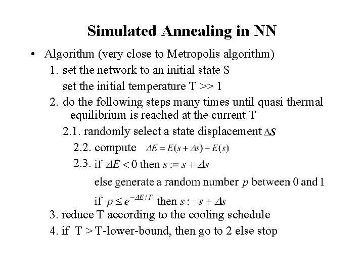
Simulated Annealing in NN • Algorithm (very close to Metropolis algorithm) 1. set the network to an initial state S set the initial temperature T >> 1 2. do the following steps many times until quasi thermal equilibrium is reached at the current T 2. 1. randomly select a state displacement 2. 2. compute 2. 3. reduce T according to the cooling schedule 4. if T > T-lower-bound, then go to 2 else stop

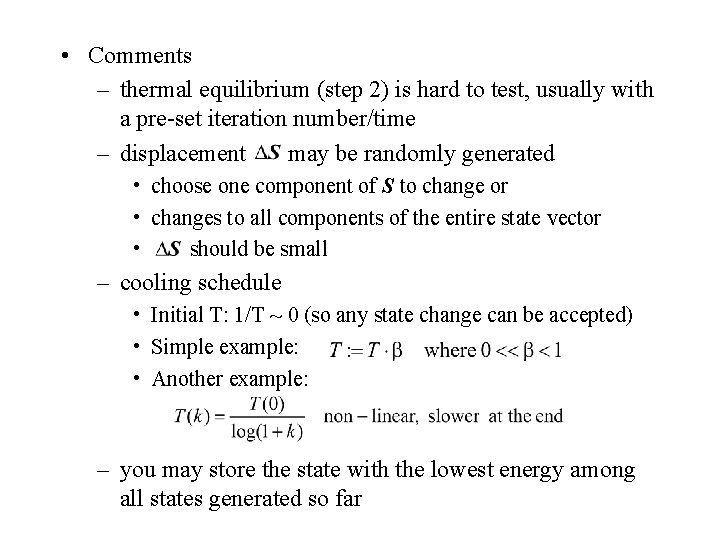
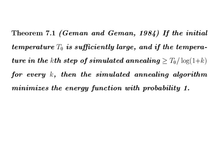
• Comments – thermal equilibrium (step 2) is hard to test, usually with a pre-set iteration number/time – displacement may be randomly generated • choose one component of S to change or • changes to all components of the entire state vector • should be small – cooling schedule • Initial T: 1/T ~ 0 (so any state change can be accepted) • Simple example: • Another example: – you may store the state with the lowest energy among all states generated so far

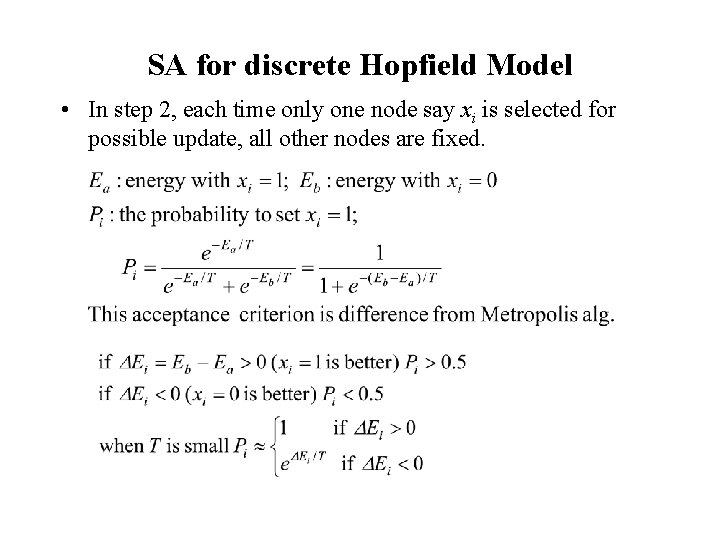
SA for discrete Hopfield Model • In step 2, each time only one node say xi is selected for possible update, all other nodes are fixed.

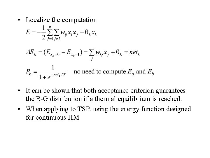
• Localize the computation • It can be shown that both acceptance criterion guarantees the B-G distribution if a thermal equilibrium is reached. • When applying to TSP, using the energy function designed for continuous HM

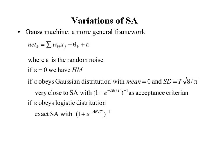
Variations of SA • Gauss machine: a more general framework

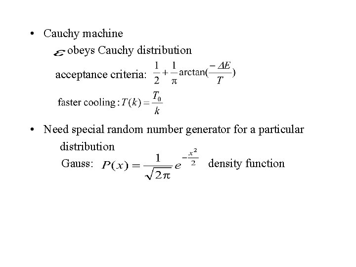
• Cauchy machine obeys Cauchy distribution acceptance criteria: • Need special random number generator for a particular distribution Gauss: density function