Oct 17 2003 MISR What determines the mean

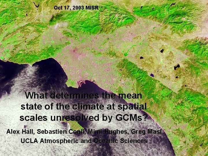
Oct 17, 2003 MISR What determines the mean state of the climate at spatial scales unresolved by GCMs? Alex Hall, Sebastien Conil, Mimi Hughes, Greg Masi UCLA Atmospheric and Oceanic Sciences

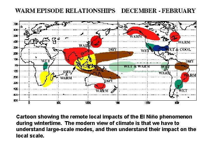
Cartoon showing the remote local impacts of the El Niño phenomenon during wintertime. The modern view of climate is that we have to understand large-scale modes, and then understand their impact on the local scale.

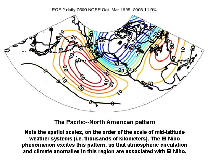
The Pacific--North American pattern Note the spatial scales, on the order of the scale of mid-latitude weather systems (i. e. thousands of kilometers). The El Niño phenomenon excites this pattern, so that atmospheric circulation and climate anomalies in this region are associated with El Niño.

Large-scale view of climate variability and change El Niño phenomenon Pacific North American pattern North Atlantic Oscillation Global climate change (increase in temperature, and intensification of the hydrologic cycle)

SIMULATING LOCAL CLIMATE

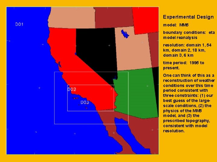
Experimental Design model: MM 5 boundary conditions: eta model reanalysis resolution: domain 1, 54 km, domain 2, 18 km, domain 3, 6 km time period: 1995 to present. One can think of this as a reconstruction of weather conditions over this time period consistent with three constraints: (1) our best guess of the largescale conditions, (2) the physics of the MM 5 model, and (3) the prescribed topography, consistent with model resolution.

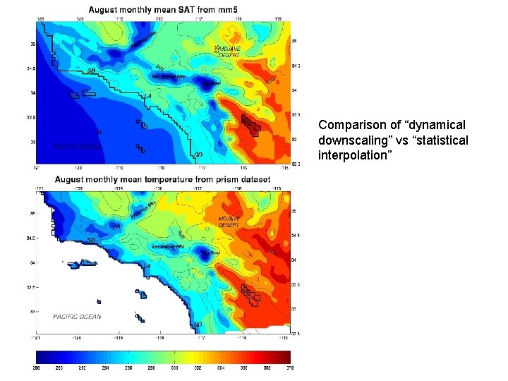
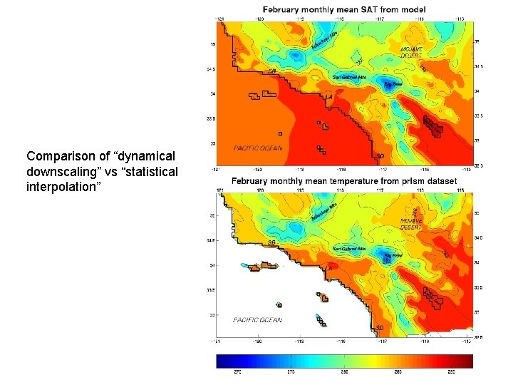
Comparison of “dynamical downscaling” vs “statistical interpolation”

Comparison of “dynamical downscaling” vs “statistical interpolation”

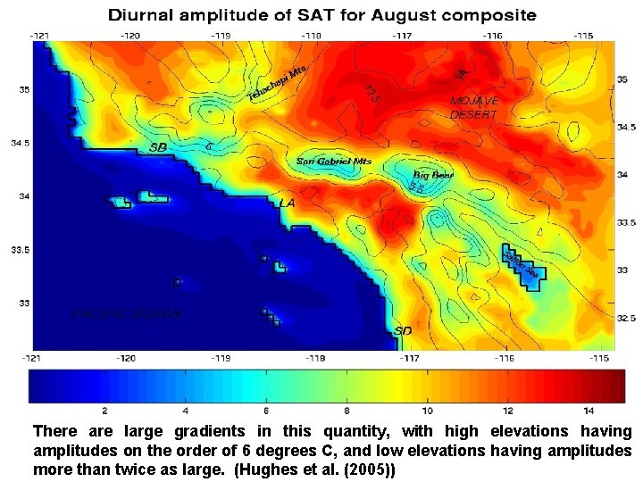
DIURNAL CYCLE AMPLITUDE

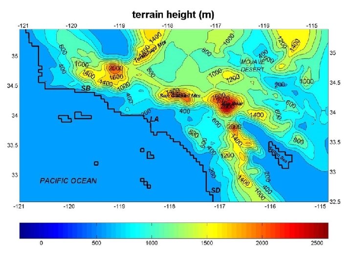
There are large gradients in this quantity, with high elevations having amplitudes on the order of 6 degrees C, and low elevations having amplitudes more than twice as large. (Hughes et al. (2005))

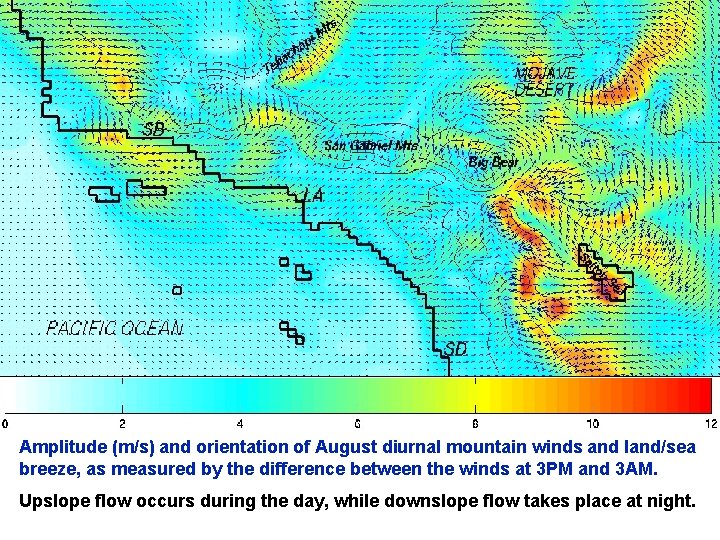
Amplitude (m/s) and orientation of August diurnal mountain winds and land/sea breeze, as measured by the difference between the winds at 3 PM and 3 AM. Upslope flow occurs during the day, while downslope flow takes place at night.

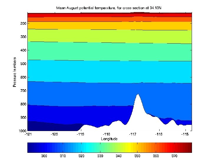
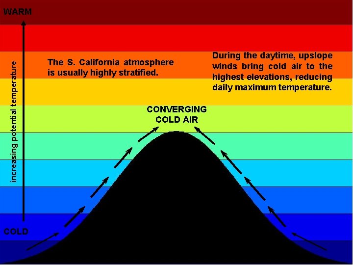
increasing potential temperature WARM COLD The S. California atmosphere is usually highly stratified. CONVERGING COLD AIR During the daytime, upslope winds bring cold air to the highest elevations, reducing daily maximum temperature.

PRECIPITATION

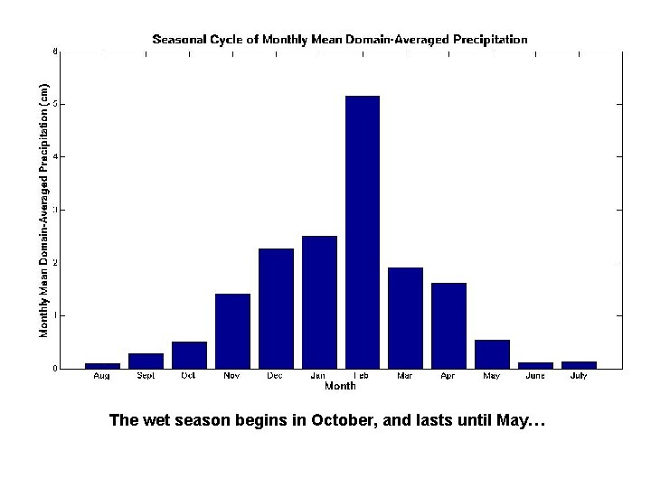
The wet season begins in October, and lasts until May…

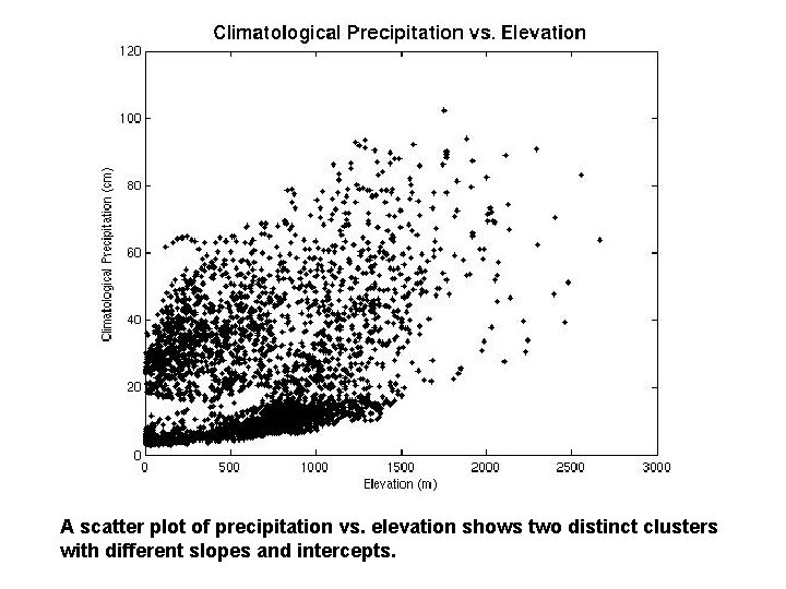
A scatter plot of precipitation vs. elevation shows two distinct clusters with different slopes and intercepts.

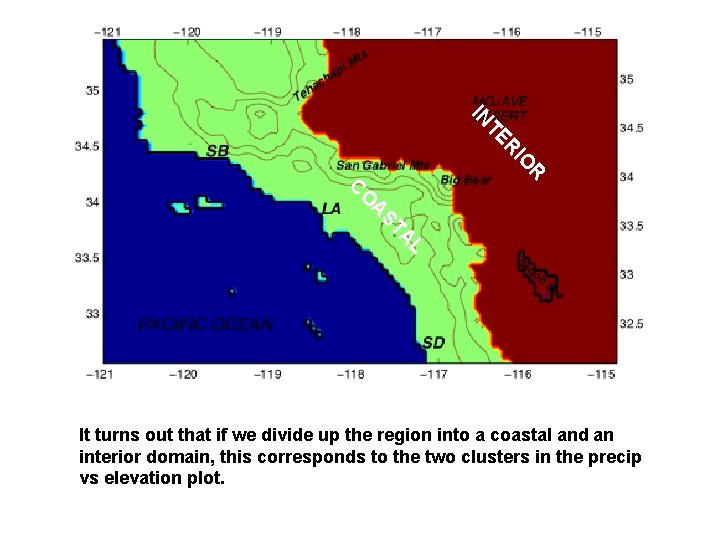
IN R IO R TE C A O L A ST It turns out that if we divide up the region into a coastal and an interior domain, this corresponds to the two clusters in the precip vs elevation plot.

A scatter plot of precipitation vs. elevation shows two distinct clusters with different slopes and intercepts.

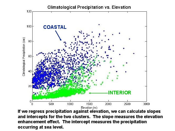
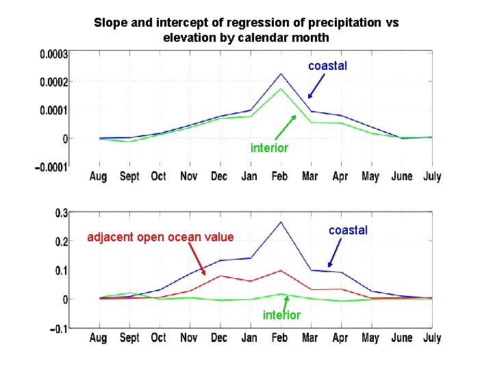
COASTAL INTERIOR If we regress precipitation against elevation, we can calculate slopes and intercepts for the two clusters. The slope measures the elevation enhancement effect. The intercept measures the precipitation occurring at sea level.

Slope and intercept of regression of precipitation vs elevation by calendar month coastal interior coastal adjacent open ocean value interior

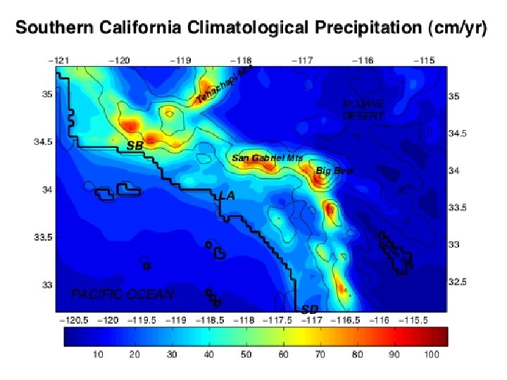
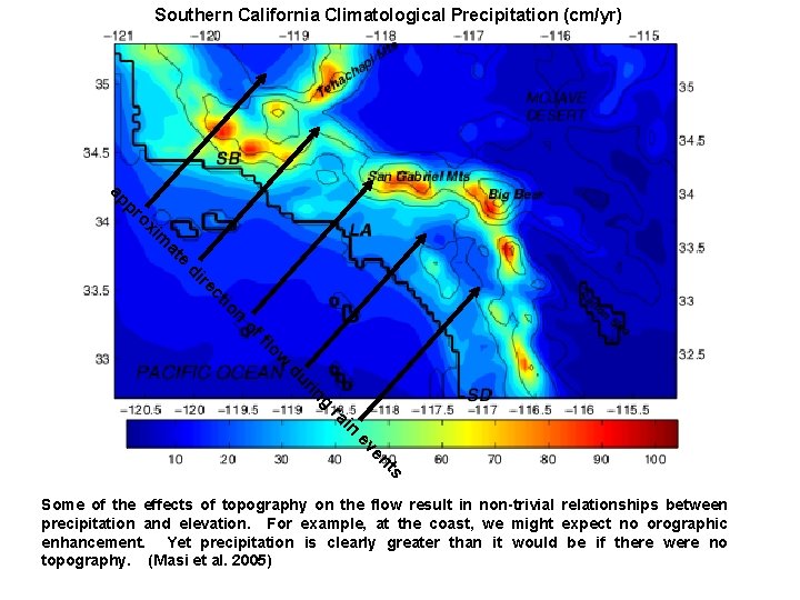
Southern California Climatological Precipitation (cm/yr) e at im ox pr ap n tio c re di of w flo du g rin in ra t en ev s Some of the effects of topography on the flow result in non-trivial relationships between precipitation and elevation. For example, at the coast, we might expect no orographic enhancement. Yet precipitation is clearly greater than it would be if there were no topography. (Masi et al. 2005)

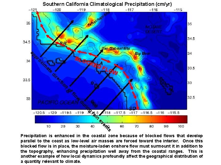
Southern California Climatological Precipitation (cm/yr) pr ap CKE DF LOW e at im ox BLO n tio c re di of w flo du g rin in ra t en ev s Precipitation is enhanced in the coastal zone because of blocked flows that develop parallel to the coast as low-level air masses are forced toward the interior. Once this blocked flow is in place, the moisture-laden onshore flow must surmount it in addition to the topography, enhancing precipitation well away from the coastal ranges. This is another example of how local dynamics profoundly affect the geographical distribution of a quantity relevant to climate.

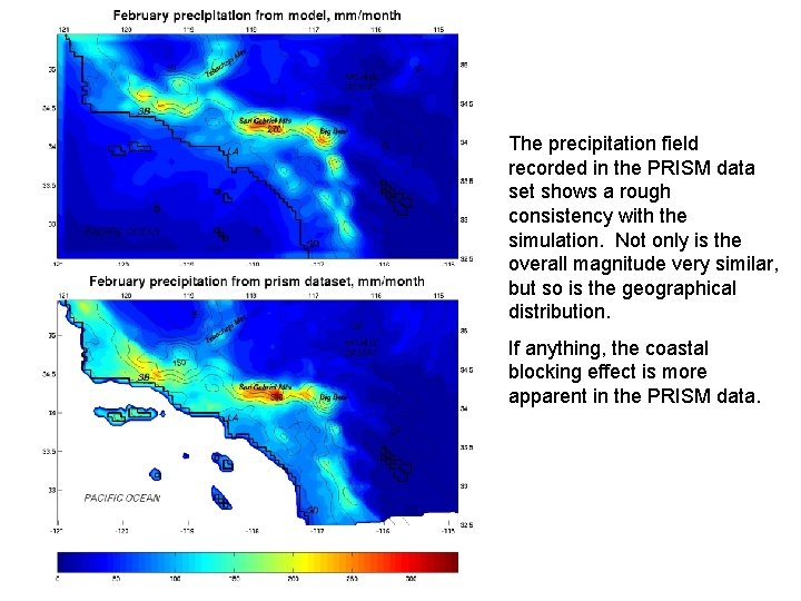
The precipitation field recorded in the PRISM data set shows a rough consistency with the simulation. Not only is the overall magnitude very similar, but so is the geographical distribution. If anything, the coastal blocking effect is more apparent in the PRISM data.

MODES OF VARIABILITY

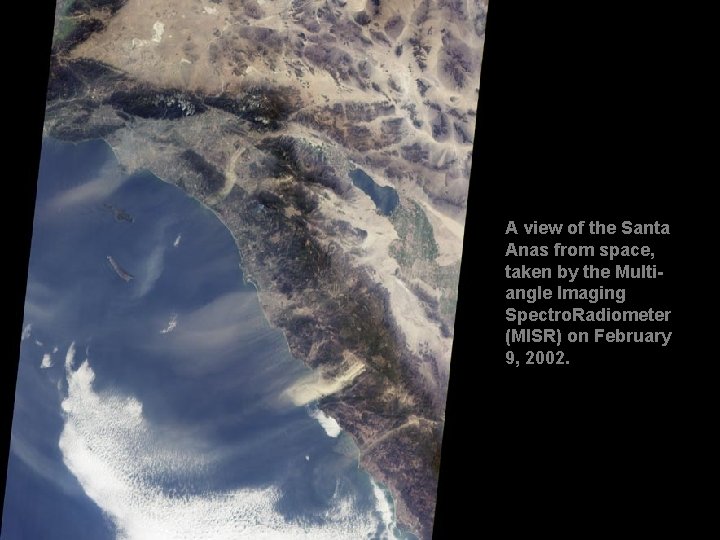
A view of the Santa Anas from space, taken by the Multiangle Imaging Spectro. Radiometer (MISR) on February 9, 2002.

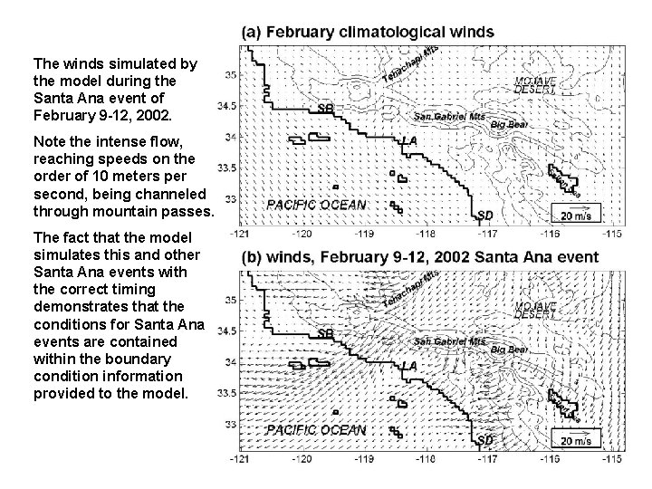
The winds simulated by the model during the Santa Ana event of February 9 -12, 2002. Note the intense flow, reaching speeds on the order of 10 meters per second, being channeled through mountain passes. The fact that the model simulates this and other Santa Ana events with the correct timing demonstrates that the conditions for Santa Ana events are contained within the boundary condition information provided to the model.

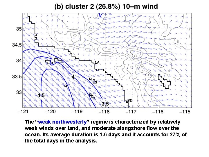
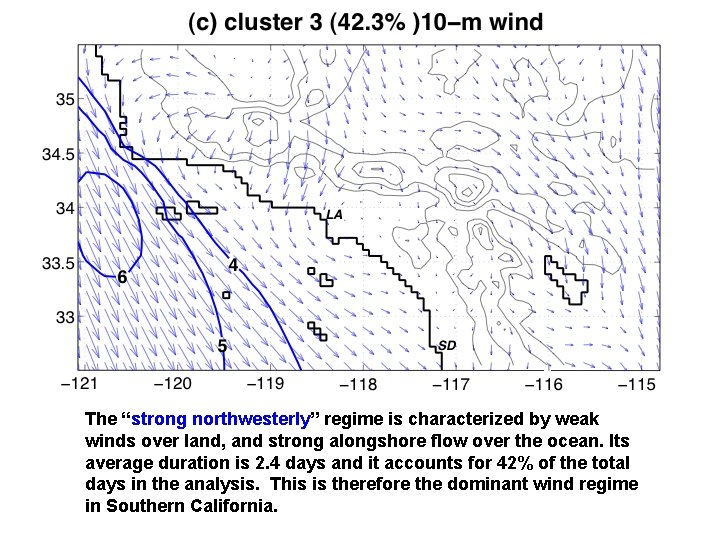
Cluster Analysis To classify the regimes of wind variability in Southern California, we performed a probabalistic cluster analysis algorithm (Smyth et al. 1999) on the October to March dailymean winds. The clustering technique provides an quantitative means of defining preferred modes of wind variability. We chose to focus on the wet season because of the interesting combination of phenomena (Santa Ana events and precipitation) during this period. We found that the wind regimes can be well-described in terms of three clusters, which together account for 82% of the days. Note that this implies that 18% of the days do not belong to any cluster, and are unclassified.

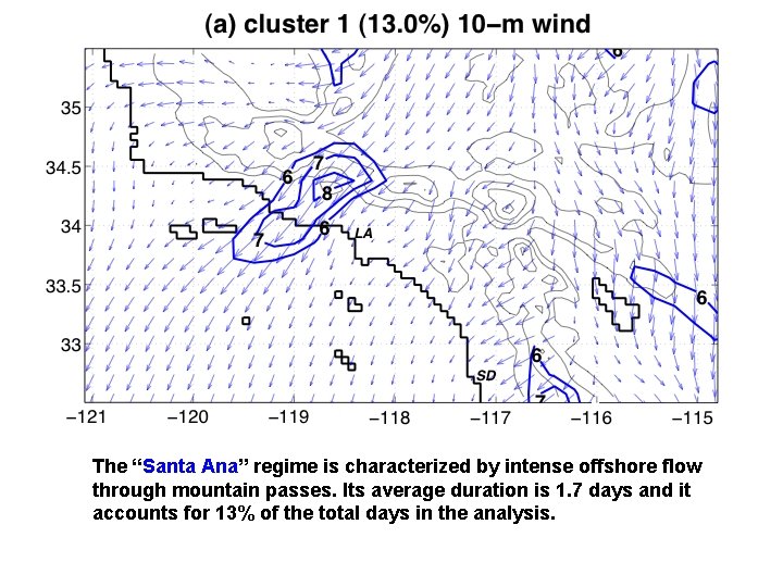
The “Santa Ana” regime is characterized by intense offshore flow through mountain passes. Its average duration is 1. 7 days and it accounts for 13% of the total days in the analysis.

The “weak northwesterly” regime is characterized by relatively weak winds over land, and moderate alongshore flow over the ocean. Its average duration is 1. 6 days and it accounts for 27% of the total days in the analysis.

The “strong northwesterly” regime is characterized by weak winds over land, and strong alongshore flow over the ocean. Its average duration is 2. 4 days and it accounts for 42% of the total days in the analysis. This is therefore the dominant wind regime in Southern California.

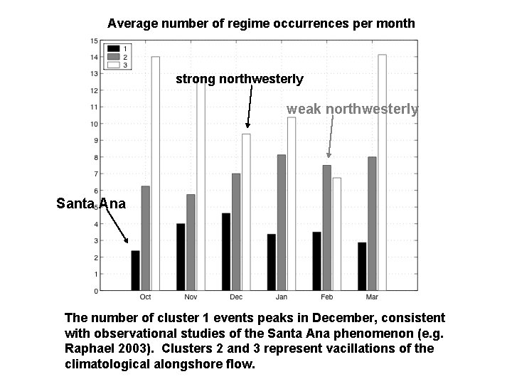
Average number of regime occurrences per month strong northwesterly weak northwesterly Santa Ana The number of cluster 1 events peaks in December, consistent with observational studies of the Santa Ana phenomenon (e. g. Raphael 2003). Clusters 2 and 3 represent vacillations of the climatological alongshore flow.

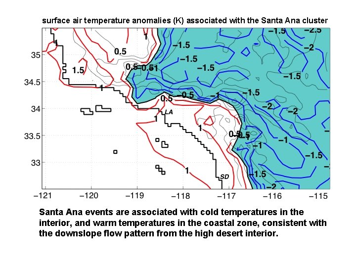
surface air temperature anomalies (K) associated with the Santa Ana cluster Santa Ana events are associated with cold temperatures in the interior, and warm temperatures in the coastal zone, consistent with the downslope flow pattern from the high desert interior.

MODES OF VARIABILITY AND HYDROLOGY

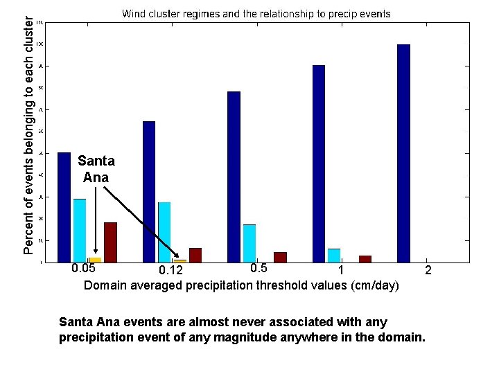
Percent of events belonging to each cluster Blah blah Santa Ana 0. 05 0. 12 1 Domain averaged precipitation threshold values (cm/day) 2 Santa Ana events are almost never associated with any precipitation event of any magnitude anywhere in the domain.

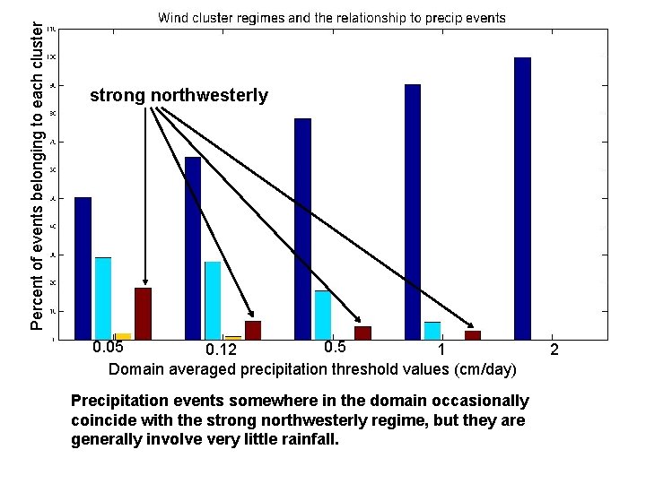
Percent of events belonging to each cluster Blah blah strong northwesterly 0. 05 0. 12 1 Domain averaged precipitation threshold values (cm/day) Precipitation events somewhere in the domain occasionally coincide with the strong northwesterly regime, but they are generally involve very little rainfall. 2

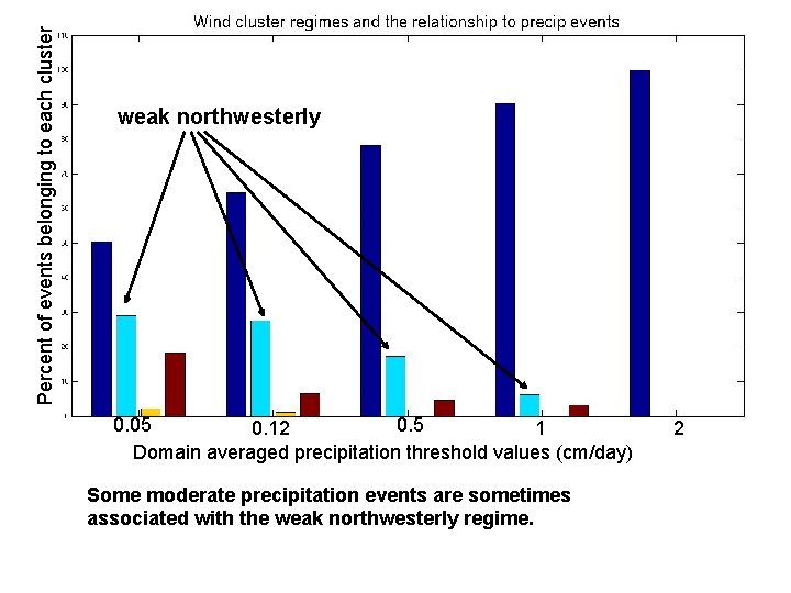
Percent of events belonging to each cluster Blah blah weak northwesterly 0. 05 0. 12 1 Domain averaged precipitation threshold values (cm/day) Some moderate precipitation events are sometimes associated with the weak northwesterly regime. 2

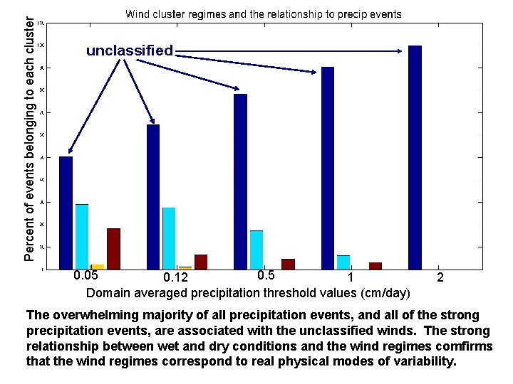
Percent of events belonging to each cluster Blah blah unclassified 0. 05 0. 12 1 Domain averaged precipitation threshold values (cm/day) 2 The overwhelming majority of all precipitation events, and all of the strong precipitation events, are associated with the unclassified winds. The strong relationship between wet and dry conditions and the wind regimes comfirms that the wind regimes correspond to real physical modes of variability.

MODES OF VARIABILITY AND THE LARGE-SCALE

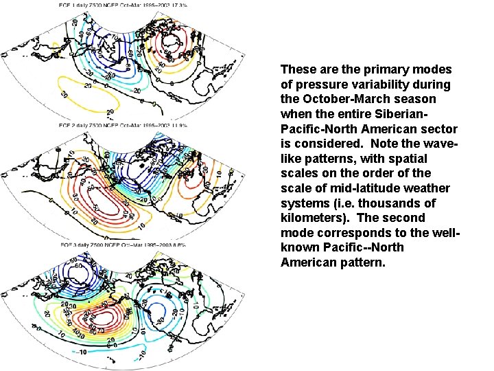
These are the primary modes of pressure variability during the October-March season when the entire Siberian. Pacific-North American sector is considered. Note the wavelike patterns, with spatial scales on the order of the scale of mid-latitude weather systems (i. e. thousands of kilometers). The second mode corresponds to the wellknown Pacific--North American pattern.

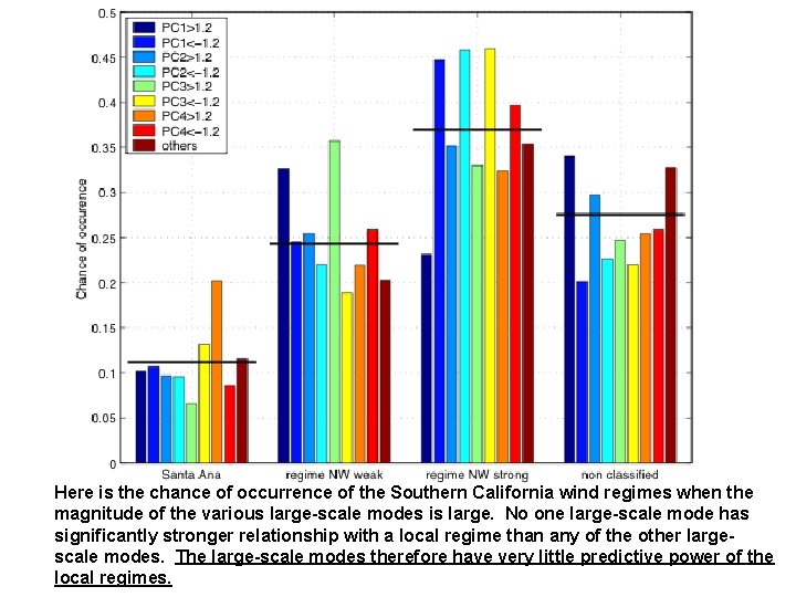
Here is the chance of occurrence of the Southern California wind regimes when the magnitude of the various large-scale modes is large. No one large-scale mode has significantly stronger relationship with a local regime than any of the other largescale modes. The large-scale modes therefore have very little predictive power of the local regimes.

A Local Perspective on Climate We show in our examination of (1) The amplitude of the diurnal cycle (2) The geographical distribution of precipitation (3) Modes of wind variability in Southern California that spatial and temporal variability in local climate is either generated by in situ by local processes, or related in a non-trivial way to the large -scale forcing. _____________ To predict climate change on spatial scales relevant for humans and ecosystems, we must understand these local processes and the complex relationships of large-scale forcing to local variability.