Multilevel Models 2 Sociology 8811 Class 24 Copyright

Multilevel Models 2 Sociology 8811, Class 24 Copyright © 2007 by Evan Schofer Do not copy or distribute without permission

Announcements • Paper #2 due in 2 weeks • Come see me ASAP if you don’t have a plan • Unfortunately, I’m unavailable during office hours today – Please send me an email to make an appointment at some other time.

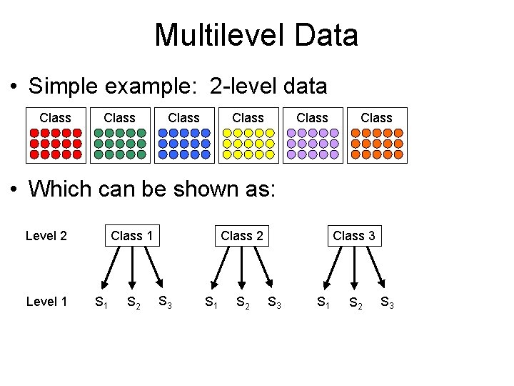
Multilevel Data • Simple example: 2 -level data Class Class • Which can be shown as: Class 1 Level 2 Level 1 S 2 Class 2 S 3 S 1 S 2 Class 3 S 1 S 2 S 3

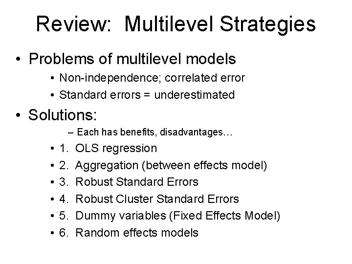
Review: Multilevel Strategies • Problems of multilevel models • Non-independence; correlated error • Standard errors = underestimated • Solutions: – Each has benefits, disadvantages… • • • 1. 2. 3. 4. 5. 6. OLS regression Aggregation (between effects model) Robust Standard Errors Robust Cluster Standard Errors Dummy variables (Fixed Effects Model) Random effects models

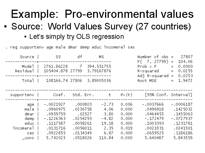
Example: Pro-environmental values • Source: World Values Survey (27 countries) • Let’s simply try OLS regression. reg supportenv age male dmar demp educ incomerel ses Source | SS df MS -------+---------------Model | 2761. 86228 7 394. 551755 Residual | 105404. 878 27799 3. 79167876 -------+---------------Total | 108166. 74 27806 3. 89005036 Number of obs F( 7, 27799) Prob > F R-squared Adj R-squared Root MSE = = = 27807 104. 06 0. 0000 0. 0255 0. 0253 1. 9472 ---------------------------------------supportenv | Coef. Std. Err. t P>|t| [95% Conf. Interval] -------+--------------------------------age | -. 0021927. 000803 -2. 73 0. 006 -. 0037666 -. 0006187 male |. 0960975. 0236758 4. 06 0. 000. 0496918. 1425032 dmar |. 0959759. 02527 3. 80 0. 000. 0464455. 1455063 demp | -. 1226363. 0254293 -4. 82 0. 000 -. 172479 -. 0727937 educ |. 1117587. 0058261 19. 18 0. 000. 1003393. 1231781 incomerel |. 0131716. 0056011 2. 35 0. 019. 0021931. 0241501 ses |. 0922855. 0134349 6. 87 0. 000. 0659525. 1186186 _cons | 5. 742023. 0518026 110. 84 0. 000 5. 640487 5. 843559

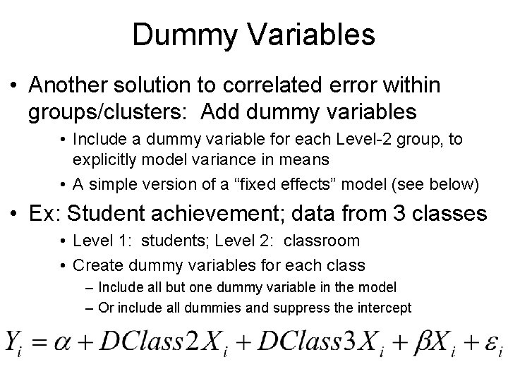
Dummy Variables • Another solution to correlated error within groups/clusters: Add dummy variables • Include a dummy variable for each Level-2 group, to explicitly model variance in means • A simple version of a “fixed effects” model (see below) • Ex: Student achievement; data from 3 classes • Level 1: students; Level 2: classroom • Create dummy variables for each class – Include all but one dummy variable in the model – Or include all dummies and suppress the intercept

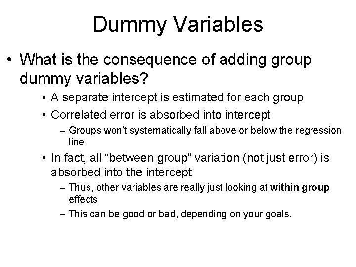
Dummy Variables • What is the consequence of adding group dummy variables? • A separate intercept is estimated for each group • Correlated error is absorbed into intercept – Groups won’t systematically fall above or below the regression line • In fact, all “between group” variation (not just error) is absorbed into the intercept – Thus, other variables are really just looking at within group effects – This can be good or bad, depending on your goals.

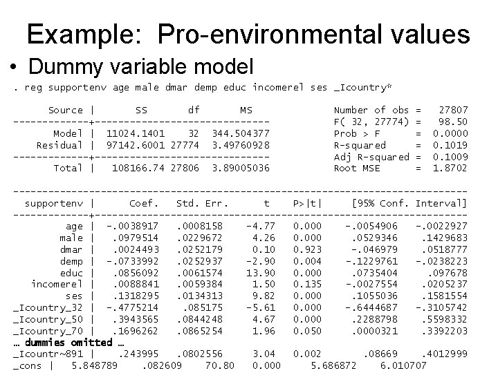
Example: Pro-environmental values • Dummy variable model. reg supportenv age male dmar demp educ incomerel ses _Icountry* Source | SS df MS -------+---------------Model | 11024. 1401 32 344. 504377 Residual | 97142. 6001 27774 3. 49760928 -------+---------------Total | 108166. 74 27806 3. 89005036 Number of obs F( 32, 27774) Prob > F R-squared Adj R-squared Root MSE = = = 27807 98. 50 0. 0000 0. 1019 0. 1009 1. 8702 ---------------------------------------supportenv | Coef. Std. Err. t P>|t| [95% Conf. Interval] -------+--------------------------------age | -. 0038917. 0008158 -4. 77 0. 000 -. 0054906 -. 0022927 male |. 0979514. 0229672 4. 26 0. 000. 0529346. 1429683 dmar |. 0024493. 0252179 0. 10 0. 923 -. 046979. 0518777 demp | -. 0733992. 0252937 -2. 90 0. 004 -. 1229761 -. 0238223 educ |. 0856092. 0061574 13. 90 0. 000. 0735404. 097678 incomerel |. 0088841. 0059384 1. 50 0. 135 -. 0027554. 0205237 ses |. 1318295. 0134313 9. 82 0. 000. 1055036. 1581554 _Icountry_32 | -. 4775214. 085175 -5. 61 0. 000 -. 6444687 -. 3105742 _Icountry_50 |. 3943565. 0844248 4. 67 0. 000. 2288798. 5598332 _Icountry_70 |. 1696262. 0865254 1. 96 0. 050. 0000321. 3392203 … dummies omitted … _Icountr~891 |. 243995. 0802556 3. 04 0. 002. 08669. 4012999 _cons | 5. 848789. 082609 70. 80 0. 000 5. 686872 6. 010707

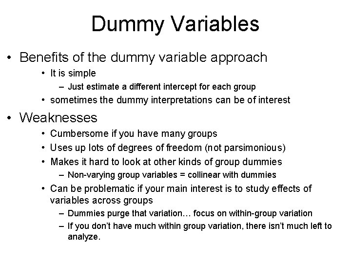
Dummy Variables • Benefits of the dummy variable approach • It is simple – Just estimate a different intercept for each group • sometimes the dummy interpretations can be of interest • Weaknesses • Cumbersome if you have many groups • Uses up lots of degrees of freedom (not parsimonious) • Makes it hard to look at other kinds of group dummies – Non-varying group variables = collinear with dummies • Can be problematic if your main interest is to study effects of variables across groups – Dummies purge that variation… focus on within-group variation – If you don’t have much within group variation, there isn’t much left to analyze.

Dummy Variables • Note: Dummy variables are a simple example of a “fixed effects” model (FEM) • Effect of each group is modeled as a “fixed effect” rather than a random variable • Also can be thought of as the “within-group” estimator – Looks purely at variation within groups – Stata can do a Fixed Effects Model without the effort of using all the dummy variables • Simply request the “fixed effects” estimator in xtreg.

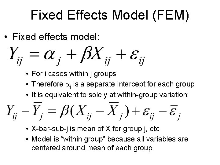
Fixed Effects Model (FEM) • Fixed effects model: • For i cases within j groups • Therefore aj is a separate intercept for each group • It is equivalent to solely at within-group variation: • X-bar-sub-j is mean of X for group j, etc • Model is “within group” because all variables are centered around mean of each group.

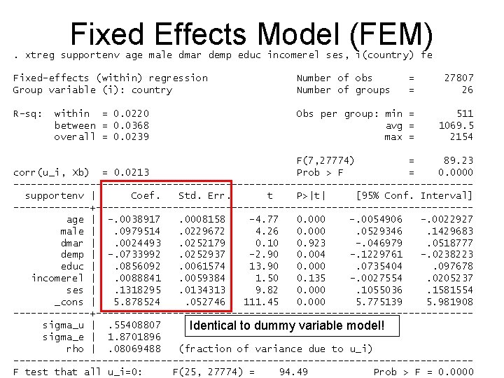
Fixed Effects Model (FEM) . xtreg supportenv age male dmar demp educ incomerel ses, i(country) fe Fixed-effects (within) regression Group variable (i): country Number of obs Number of groups = = 27807 26 R-sq: Obs per group: min = avg = max = 511 1069. 5 2154 within = 0. 0220 between = 0. 0368 overall = 0. 0239 F(7, 27774) = 89. 23 corr(u_i, Xb) = 0. 0213 Prob > F = 0. 0000 ---------------------------------------supportenv | Coef. Std. Err. t P>|t| [95% Conf. Interval] -------+--------------------------------age | -. 0038917. 0008158 -4. 77 0. 000 -. 0054906 -. 0022927 male |. 0979514. 0229672 4. 26 0. 000. 0529346. 1429683 dmar |. 0024493. 0252179 0. 10 0. 923 -. 046979. 0518777 demp | -. 0733992. 0252937 -2. 90 0. 004 -. 1229761 -. 0238223 educ |. 0856092. 0061574 13. 90 0. 000. 0735404. 097678 incomerel |. 0088841. 0059384 1. 50 0. 135 -. 0027554. 0205237 ses |. 1318295. 0134313 9. 82 0. 000. 1055036. 1581554 _cons | 5. 878524. 052746 111. 45 0. 000 5. 775139 5. 981908 -------+--------------------------------sigma_u |. 55408807 Identical to dummy variable model! sigma_e | 1. 8701896 rho |. 08069488 (fraction of variance due to u_i) ---------------------------------------F test that all u_i=0: F(25, 27774) = 94. 49 Prob > F = 0. 0000

ANOVA: A Digression • Suppose you wish to model variable Y for j groups (clusters) • Ex: Wages for different racial groups • Definitions: • The grand mean is the mean of all groups – Y-bar • The group mean is the mean of a particular sub-group of the population – Y-bar-sub-j

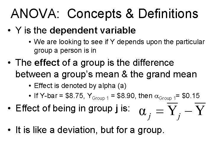
ANOVA: Concepts & Definitions • Y is the dependent variable • We are looking to see if Y depends upon the particular group a person is in • The effect of a group is the difference between a group’s mean & the grand mean • Effect is denoted by alpha (a) • If Y-bar = $8. 75, YGroup 1 = $8. 90, then a. Group 1= $0. 15 • Effect of being in group j is: • It is like a deviation, but for a group.

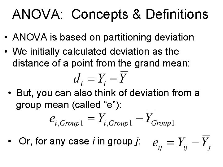
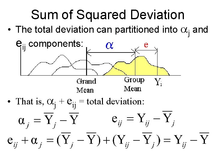
ANOVA: Concepts & Definitions • ANOVA is based on partitioning deviation • We initially calculated deviation as the distance of a point from the grand mean: • But, you can also think of deviation from a group mean (called “e”): • Or, for any case i in group j:

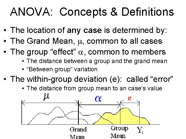
ANOVA: Concepts & Definitions • The location of any case is determined by: • The Grand Mean, m, common to all cases • The group “effect” a, common to members • The distance between a group and the grand mean • “Between group” variation • The within-group deviation (e): called “error” • The distance from group mean to an case’s value

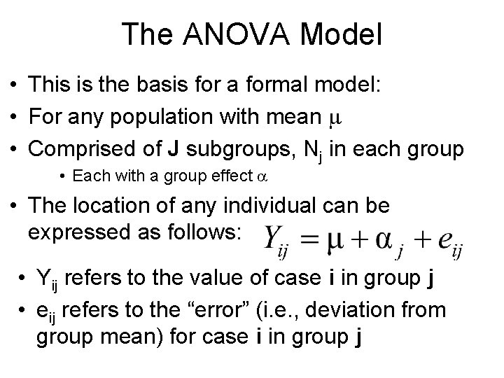
The ANOVA Model • This is the basis for a formal model: • For any population with mean m • Comprised of J subgroups, Nj in each group • Each with a group effect a • The location of any individual can be expressed as follows: • Yij refers to the value of case i in group j • eij refers to the “error” (i. e. , deviation from group mean) for case i in group j

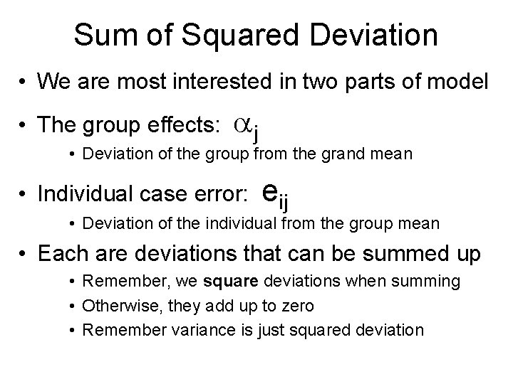
Sum of Squared Deviation • We are most interested in two parts of model • The group effects: aj • Deviation of the group from the grand mean • Individual case error: eij • Deviation of the individual from the group mean • Each are deviations that can be summed up • Remember, we square deviations when summing • Otherwise, they add up to zero • Remember variance is just squared deviation

Sum of Squared Deviation • The total deviation can partitioned into aj and eij components: • That is, aj + eij = total deviation:

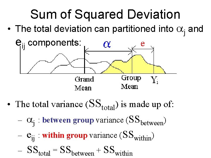
Sum of Squared Deviation • The total deviation can partitioned into aj and eij components: • The total variance (SStotal) is made up of: – – – aj : between group variance (SSbetween) eij : within group variance (SSwithin) SStotal = SSbetween + SSwithin

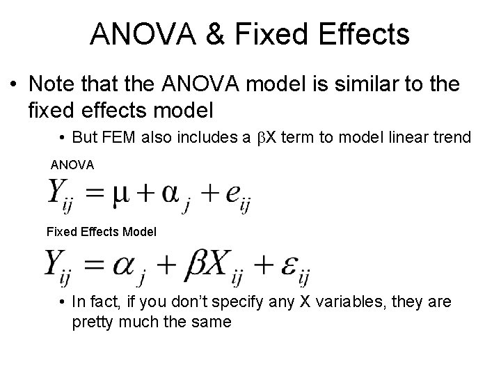
ANOVA & Fixed Effects • Note that the ANOVA model is similar to the fixed effects model • But FEM also includes a b. X term to model linear trend ANOVA Fixed Effects Model • In fact, if you don’t specify any X variables, they are pretty much the same

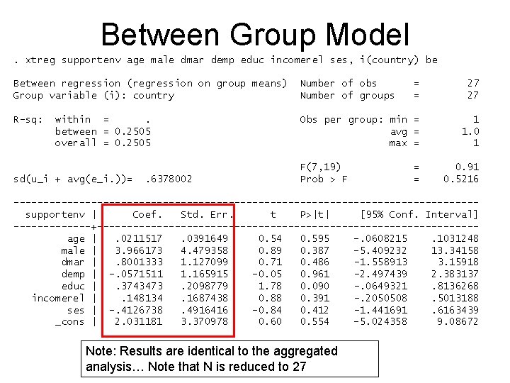
Within Group & Between Group Models • Group-effect dummy variables in regression model creates a specific estimate of group effects for all cases • Bs & error are based on remaining “within group” variation • We could do the opposite: ignore within-group variation and just look at differences between • Stata’s xtreg command can do this, too • This is essentially just modeling group means!

Between Group Model. xtreg supportenv age male dmar demp educ incomerel ses, i(country) be Between regression (regression on group means) Group variable (i): country Number of obs Number of groups = = 27 27 R-sq: Obs per group: min = avg = max = 1 1. 0 1 within =. between = 0. 2505 overall = 0. 2505 sd(u_i + avg(e_i. ))= . 6378002 F(7, 19) Prob > F = = 0. 91 0. 5216 ---------------------------------------supportenv | Coef. Std. Err. t P>|t| [95% Conf. Interval] -------+--------------------------------age |. 0211517. 0391649 0. 54 0. 595 -. 0608215. 1031248 male | 3. 966173 4. 479358 0. 89 0. 387 -5. 409232 13. 34158 dmar |. 8001333 1. 127099 0. 71 0. 486 -1. 558913 3. 15918 demp | -. 0571511 1. 165915 -0. 05 0. 961 -2. 497439 2. 383137 educ |. 3743473. 2098779 1. 78 0. 090 -. 0649321. 8136268 incomerel |. 148134. 1687438 0. 88 0. 391 -. 2050508. 5013188 ses | -. 4126738. 4916416 -0. 84 0. 412 -1. 441691. 6163439 _cons | 2. 031181 3. 370978 0. 60 0. 554 -5. 024358 9. 08672 Note: Results are identical to the aggregated analysis… Note that N is reduced to 27

Fixed vs. Random Effects • Dummy variables produce a “fixed” estimate of the intercept for each group • But, models don’t need to be based on fixed effects • Example: The error term (ei) • We could estimate a fixed value for all cases – This would use up lots of degrees of freedom – even more than using group dummies • In fact, we would use up ALL degrees of freedom – Stata output would simply report back the raw data (expressed as deviations from the constant) • Instead, we model e as a random variable – We assume it is normal, with standard deviation sigma.

Random Effects • Issue: The dummy variable approach (ANOVA, FEM) treats group differences as a fixed effect • Alternatively, we can treat it as a random effect • Don’t estimate values for each case, but model it • This requires making assumptions – e. g. , that group differences are normally distributed with a standard deviation that can be estimated from data

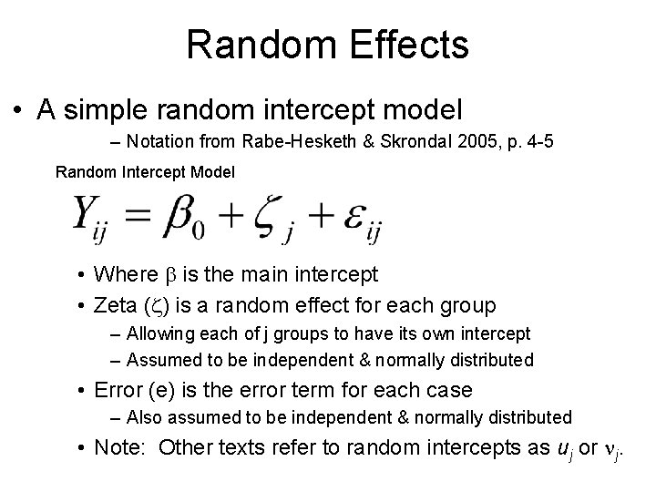
Random Effects • A simple random intercept model – Notation from Rabe-Hesketh & Skrondal 2005, p. 4 -5 Random Intercept Model • Where b is the main intercept • Zeta (z) is a random effect for each group – Allowing each of j groups to have its own intercept – Assumed to be independent & normally distributed • Error (e) is the error term for each case – Also assumed to be independent & normally distributed • Note: Other texts refer to random intercepts as uj or nj.

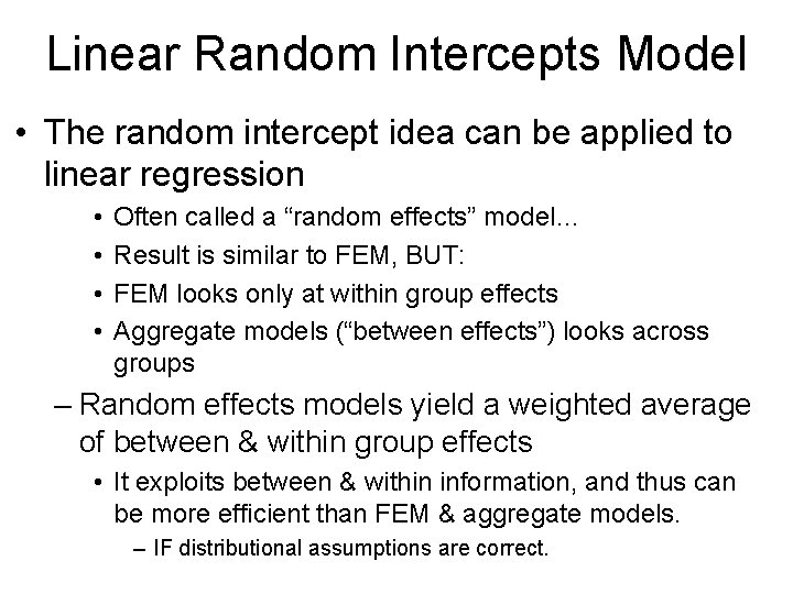
Linear Random Intercepts Model • The random intercept idea can be applied to linear regression • • Often called a “random effects” model… Result is similar to FEM, BUT: FEM looks only at within group effects Aggregate models (“between effects”) looks across groups – Random effects models yield a weighted average of between & within group effects • It exploits between & within information, and thus can be more efficient than FEM & aggregate models. – IF distributional assumptions are correct.

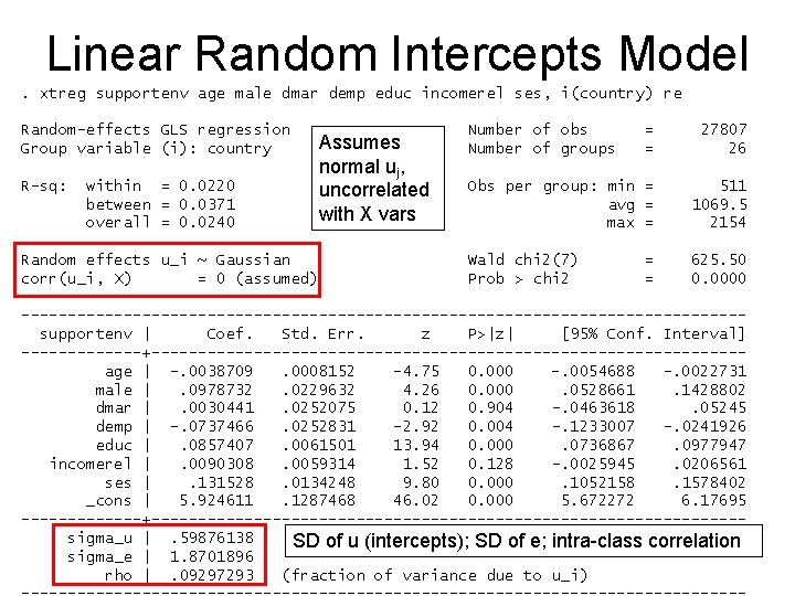
Linear Random Intercepts Model. xtreg supportenv age male dmar demp educ incomerel ses, i(country) re Random-effects GLS regression Group variable (i): country R-sq: within = 0. 0220 between = 0. 0371 overall = 0. 0240 Random effects u_i ~ Gaussian corr(u_i, X) = 0 (assumed) Assumes normal uj, uncorrelated with X vars Number of obs Number of groups = = 27807 26 Obs per group: min = avg = max = 511 1069. 5 2154 Wald chi 2(7) Prob > chi 2 625. 50 0. 0000 = = ---------------------------------------supportenv | Coef. Std. Err. z P>|z| [95% Conf. Interval] -------+--------------------------------age | -. 0038709. 0008152 -4. 75 0. 000 -. 0054688 -. 0022731 male |. 0978732. 0229632 4. 26 0. 000. 0528661. 1428802 dmar |. 0030441. 0252075 0. 12 0. 904 -. 0463618. 05245 demp | -. 0737466. 0252831 -2. 92 0. 004 -. 1233007 -. 0241926 educ |. 0857407. 0061501 13. 94 0. 000. 0736867. 0977947 incomerel |. 0090308. 0059314 1. 52 0. 128 -. 0025945. 0206561 ses |. 131528. 0134248 9. 80 0. 000. 1052158. 1578402 _cons | 5. 924611. 1287468 46. 02 0. 000 5. 672272 6. 17695 -------+--------------------------------sigma_u |. 59876138 SD of u (intercepts); SD of e; intra-class correlation sigma_e | 1. 8701896 rho |. 09297293 (fraction of variance due to u_i)

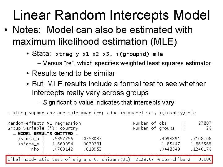
Linear Random Intercepts Model • Notes: Model can also be estimated with maximum likelihood estimation (MLE) • Stata: xtreg y x 1 x 2 x 3, i(groupid) mle – Versus “re”, which specifies weighted least squares estimator • Results tend to be similar • But, MLE results include a formal test to see whether intercepts really vary across groups – Significant p-value indicates that intercepts vary. xtreg supportenv age male dmar demp educ incomerel ses, i(country) mle Random-effects ML regression Number of obs = 27807 Group variable (i): country Number of groups = 26 … MODEL RESULTS OMITTED … /sigma_u |. 5397755. 0758087. 4098891. 7108206 /sigma_e | 1. 869954. 0079331 1. 85447 1. 885568 rho |. 0769142. 019952. 0448349. 1240176 ---------------------------------------Likelihood-ratio test of sigma_u=0: chibar 2(01)= 2128. 07 Prob>=chibar 2 = 0. 000

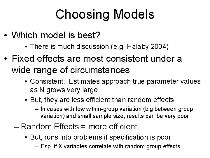
Choosing Models • Which model is best? • There is much discussion (e. g, Halaby 2004) • Fixed effects are most consistent under a wide range of circumstances • Consistent: Estimates approach true parameter values as N grows very large • But, they are less efficient than random effects – In cases with low within-group variation (big between group variation) and small sample size, results can be very poor – Random Effects = more efficient • But, runs into problems if specification is poor – Esp. if X variables correlate with random group effects.

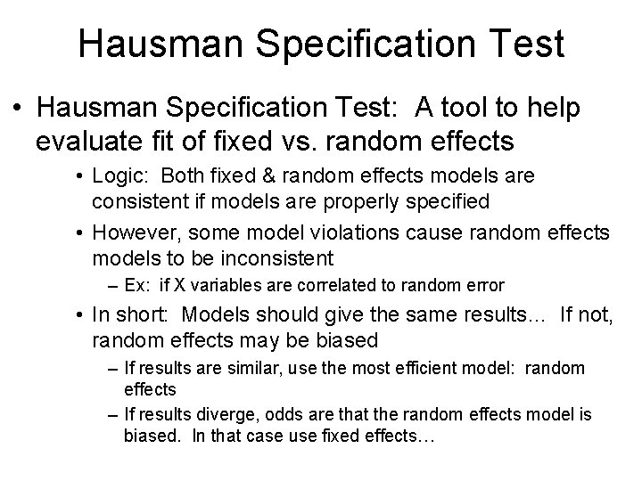
Hausman Specification Test • Hausman Specification Test: A tool to help evaluate fit of fixed vs. random effects • Logic: Both fixed & random effects models are consistent if models are properly specified • However, some model violations cause random effects models to be inconsistent – Ex: if X variables are correlated to random error • In short: Models should give the same results… If not, random effects may be biased – If results are similar, use the most efficient model: random effects – If results diverge, odds are that the random effects model is biased. In that case use fixed effects…

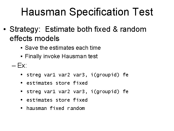
Hausman Specification Test • Strategy: Estimate both fixed & random effects models • Save the estimates each time • Finally invoke Hausman test – Ex: • • • streg var 1 var 2 var 3, i(groupid) fe estimates store fixed hausman fixed random

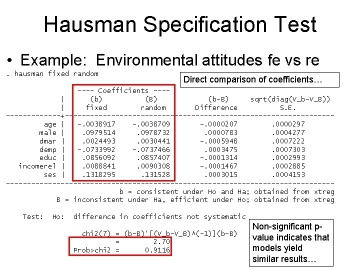
Hausman Specification Test • Example: Environmental attitudes fe vs re. hausman fixed random Direct comparison of coefficients… ---- Coefficients ---| (b) (B) (b-B) sqrt(diag(V_b-V_B)) | fixed random Difference S. E. -------+--------------------------------age | -. 0038917 -. 0038709 -. 0000207. 0000297 male |. 0979514. 0978732. 0000783. 0004277 dmar |. 0024493. 0030441 -. 0005948. 0007222 demp | -. 0733992 -. 0737466. 0003475. 0007303 educ |. 0856092. 0857407 -. 0001314. 0002993 incomerel |. 0088841. 0090308 -. 0001467. 0002885 ses |. 1318295. 131528. 0003015. 0004153 ---------------------------------------b = consistent under Ho and Ha; obtained from xtreg B = inconsistent under Ha, efficient under Ho; obtained from xtreg Test: Ho: difference in coefficients not systematic chi 2(7) = (b-B)'[(V_b-V_B)^(-1)](b-B) = 2. 70 Prob>chi 2 = 0. 9116 Non-significant pvalue indicates that models yield similar results…