Multilevel Models 3 Sociology 8811 Class 25 Copyright

Multilevel Models 3 Sociology 8811, Class 25 Copyright © 2007 by Evan Schofer Do not copy or distribute without permission

Announcements • Paper #2 due April 26 • Come see me ASAP if you don’t have a plan – Class topic: More multilevel models

Paper #1 Comments • Papers were very good overall! • Main issues: – 1. A few people didn’t devote much time to diagnostics… they are important! – 2. Some issues with models… choice of variables needs to be thought through – 3. Some issues with focus / attention • Don’t spend 2 pages describing the histogram of each and every variable • Prioritize! Focus on interesting / important things – Ex: spend more time on problematic diagnostics, less on unimportant detail

Paper #1 Comments • Main issues: – 4. Avoid obviously useless plots/diagrams/info • Ex: useless scatterplots of nominal/ordinal variables (without jitter) – 5. Avoid over-strong / absolute language • “There were no standardized residuals over 3, so I was able to determine that there were no outliers. ” – First, standardized residuals is not the best way to diagnose outliers. Cooks D and other statistics help paint a full picture. – Second, (and more importantly): conclusion is too strong – Better to say: Examination of standardized residuals, cooks D, and scatterplots found no indication of influential cases.

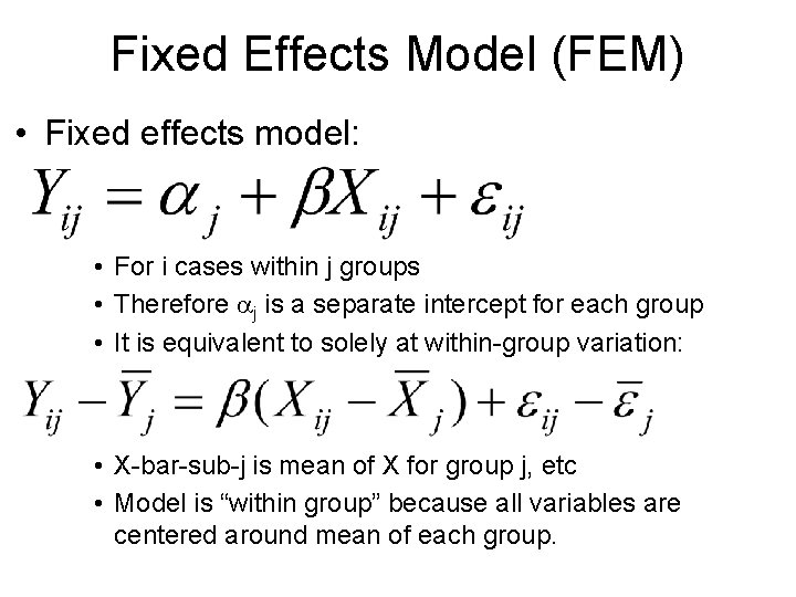
Fixed Effects Model (FEM) • Fixed effects model: • For i cases within j groups • Therefore aj is a separate intercept for each group • It is equivalent to solely at within-group variation: • X-bar-sub-j is mean of X for group j, etc • Model is “within group” because all variables are centered around mean of each group.

Random Effects • Issue: The dummy variable approach (ANOVA, FEM) treats group differences as a fixed effect • Alternatively, we can treat it as a random effect • Don’t estimate values for each case, but model it • This requires making assumptions – e. g. , that group differences are normally distributed with a standard deviation that can be estimated from data.

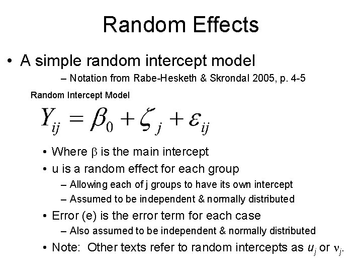
Random Effects • A simple random intercept model – Notation from Rabe-Hesketh & Skrondal 2005, p. 4 -5 Random Intercept Model • Where b is the main intercept • u is a random effect for each group – Allowing each of j groups to have its own intercept – Assumed to be independent & normally distributed • Error (e) is the error term for each case – Also assumed to be independent & normally distributed • Note: Other texts refer to random intercepts as uj or nj.

Linear Random Intercepts Model • The random intercept idea can be applied to linear regression • • Often called a “random effects” model… Result is similar to FEM, BUT: FEM looks only at within group effects Aggregate models (“between effects”) looks across groups – Random effects models yield a weighted average of between & within group effects • It exploits between & within information, and thus can be more efficient than FEM & aggregate models. – IF distributional assumptions are correct.

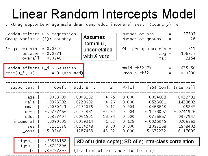
Linear Random Intercepts Model. xtreg supportenv age male dmar demp educ incomerel ses, i(country) re Random-effects GLS regression Group variable (i): country R-sq: within = 0. 0220 between = 0. 0371 overall = 0. 0240 Random effects u_i ~ Gaussian corr(u_i, X) = 0 (assumed) Assumes normal uj, uncorrelated with X vars Number of obs Number of groups = = 27807 26 Obs per group: min = avg = max = 511 1069. 5 2154 Wald chi 2(7) Prob > chi 2 625. 50 0. 0000 = = ---------------------------------------supportenv | Coef. Std. Err. z P>|z| [95% Conf. Interval] -------+--------------------------------age | -. 0038709. 0008152 -4. 75 0. 000 -. 0054688 -. 0022731 male |. 0978732. 0229632 4. 26 0. 000. 0528661. 1428802 dmar |. 0030441. 0252075 0. 12 0. 904 -. 0463618. 05245 demp | -. 0737466. 0252831 -2. 92 0. 004 -. 1233007 -. 0241926 educ |. 0857407. 0061501 13. 94 0. 000. 0736867. 0977947 incomerel |. 0090308. 0059314 1. 52 0. 128 -. 0025945. 0206561 ses |. 131528. 0134248 9. 80 0. 000. 1052158. 1578402 _cons | 5. 924611. 1287468 46. 02 0. 000 5. 672272 6. 17695 -------+--------------------------------sigma_u |. 59876138 SD of u (intercepts); SD of e; intra-class correlation sigma_e | 1. 8701896 rho |. 09297293 (fraction of variance due to u_i)

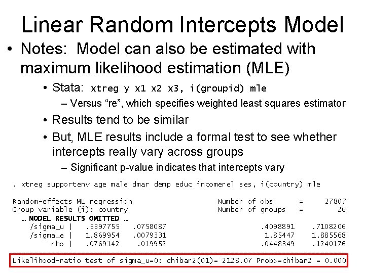
Linear Random Intercepts Model • Notes: Model can also be estimated with maximum likelihood estimation (MLE) • Stata: xtreg y x 1 x 2 x 3, i(groupid) mle – Versus “re”, which specifies weighted least squares estimator • Results tend to be similar • But, MLE results include a formal test to see whether intercepts really vary across groups – Significant p-value indicates that intercepts vary. xtreg supportenv age male dmar demp educ incomerel ses, i(country) mle Random-effects ML regression Number of obs = 27807 Group variable (i): country Number of groups = 26 … MODEL RESULTS OMITTED … /sigma_u |. 5397755. 0758087. 4098891. 7108206 /sigma_e | 1. 869954. 0079331 1. 85447 1. 885568 rho |. 0769142. 019952. 0448349. 1240176 ---------------------------------------Likelihood-ratio test of sigma_u=0: chibar 2(01)= 2128. 07 Prob>=chibar 2 = 0. 000

Choosing Models • Which model is best? • There is much discussion (e. g, Halaby 2004) • Fixed effects are most consistent under a wide range of circumstances • Consistent: Estimates approach true parameter values as N grows very large • But, they are less efficient than random effects – In cases with low within-group variation (big between group variation) and small sample size, results can be very poor – Random Effects = more efficient • But, runs into problems if specification is poor – Esp. if X variables correlate with random group effects – Usually due to omitted variables.

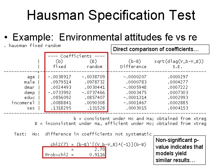
Hausman Specification Test • Hausman Specification Test: A tool to help evaluate fit of fixed vs. random effects • Logic: Both fixed & random effects models are consistent if models are properly specified • However, some model violations cause random effects models to be inconsistent – Ex: if X variables are correlated to random error • In short: Models should give the same results… If not, random effects may be biased – If results are similar, use the most efficient model: random effects – If results diverge, odds are that the random effects model is biased. In that case use fixed effects…

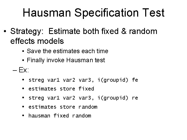
Hausman Specification Test • Strategy: Estimate both fixed & random effects models • Save the estimates each time • Finally invoke Hausman test – Ex: • • • streg var 1 var 2 var 3, i(groupid) fe estimates store fixed streg var 1 var 2 var 3, i(groupid) re estimates store random hausman fixed random

Hausman Specification Test • Example: Environmental attitudes fe vs re. hausman fixed random Direct comparison of coefficients… ---- Coefficients ---| (b) (B) (b-B) sqrt(diag(V_b-V_B)) | fixed random Difference S. E. -------+--------------------------------age | -. 0038917 -. 0038709 -. 0000207. 0000297 male |. 0979514. 0978732. 0000783. 0004277 dmar |. 0024493. 0030441 -. 0005948. 0007222 demp | -. 0733992 -. 0737466. 0003475. 0007303 educ |. 0856092. 0857407 -. 0001314. 0002993 incomerel |. 0088841. 0090308 -. 0001467. 0002885 ses |. 1318295. 131528. 0003015. 0004153 ---------------------------------------b = consistent under Ho and Ha; obtained from xtreg B = inconsistent under Ha, efficient under Ho; obtained from xtreg Test: Ho: difference in coefficients not systematic chi 2(7) = (b-B)'[(V_b-V_B)^(-1)](b-B) = 2. 70 Prob>chi 2 = 0. 9116 Non-significant pvalue indicates that models yield similar results…

Within & Between Effects • What is the relationship between within-group effects (FEM) and between-effects (BEM)? • • Usually they are similar Ex: Student skills & test performance Within any classroom, skilled students do best on tests Between classrooms, classes with more skilled students have higher mean test scores.

Within & Between Effects • Issue: Between and within effects can differ! • Ex: Effects of wealth on attitudes toward welfare • At the individual level (within group) – Wealthier people are conservative, don’t support welfare • At the country level (between groups): – Wealthier countries (high aggregate mean) tend to have prowelfare attitudes (ex: Scandinavia) • Result: Wealth has opposite between vs within effects! – Issue: Such dynamics often result from omitted level-1 variables (omitted variable bias) • Ex: If we control for individual “political conservatism”, effects may be consistent at both levels…

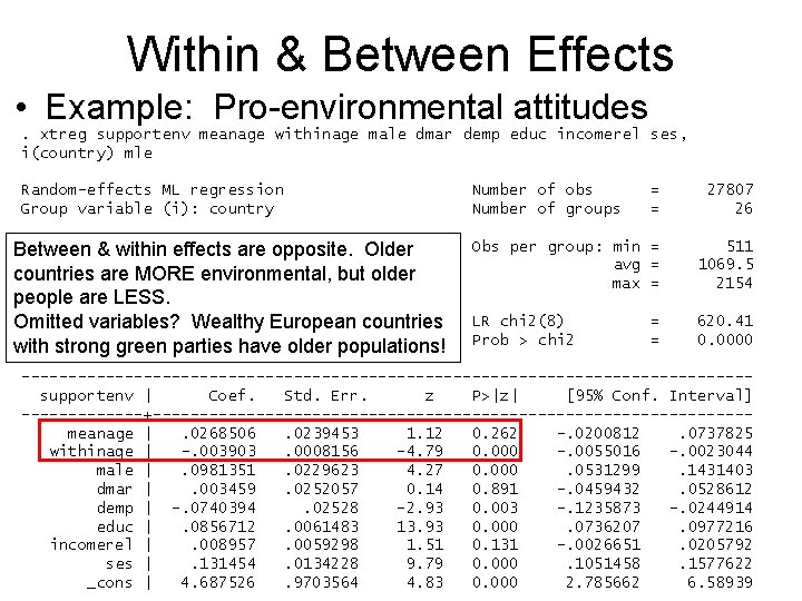
Within & Between Effects • You can estimate BOTH within- and betweengroup effects in a single model • Strategy: Split a variable (e. g. , SES) into two new variables… – 1. Group mean SES – 2. Within-group deviation from mean SES » Often called “group mean centering” • Then, put both variables into a random effects model • Model will estimate separate coefficients for between vs. within effects – Ex: • egen meanvar 1 = mean(var 1), by(groupid) • egen withinvar 1 = var 1 – meanvar 1 • Include mean (aggregate) & within variable in model.

Within & Between Effects • Example: Pro-environmental attitudes. xtreg supportenv meanage withinage male dmar demp educ incomerel ses, i(country) mle Random-effects ML regression Group variable (i): country Random effects ~ Gaussian Between & withinu_i effects are opposite. Older countries are MORE environmental, but older people are LESS. Omitted variables? Wealthy European countries Log strong likelihood -56918. 299 with green =parties have older populations! Number of obs Number of groups = = 27807 26 Obs per group: min = avg = max = 511 1069. 5 2154 LR chi 2(8) Prob > chi 2 620. 41 0. 0000 = = ---------------------------------------supportenv | Coef. Std. Err. z P>|z| [95% Conf. Interval] -------+--------------------------------meanage |. 0268506. 0239453 1. 12 0. 262 -. 0200812. 0737825 withinage | -. 003903. 0008156 -4. 79 0. 000 -. 0055016 -. 0023044 male |. 0981351. 0229623 4. 27 0. 000. 0531299. 1431403 dmar |. 003459. 0252057 0. 14 0. 891 -. 0459432. 0528612 demp | -. 0740394. 02528 -2. 93 0. 003 -. 1235873 -. 0244914 educ |. 0856712. 0061483 13. 93 0. 000. 0736207. 0977216 incomerel |. 008957. 0059298 1. 51 0. 131 -. 0026651. 0205792 ses |. 131454. 0134228 9. 79 0. 000. 1051458. 1577622 _cons | 4. 687526. 9703564 4. 83 0. 000 2. 785662 6. 58939

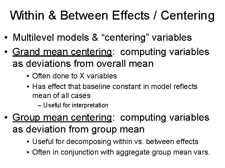
Within & Between Effects / Centering • Multilevel models & “centering” variables • Grand mean centering: computing variables as deviations from overall mean • Often done to X variables • Has effect that baseline constant in model reflects mean of all cases – Useful for interpretation • Group mean centering: computing variables as deviation from group mean • Useful for decomposing within vs. between effects • Often in conjunction with aggregate group mean vars.

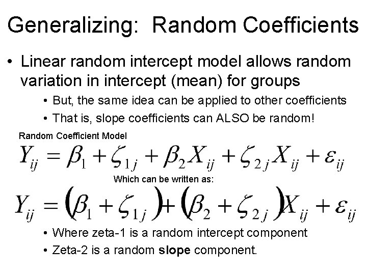
Generalizing: Random Coefficients • Linear random intercept model allows random variation in intercept (mean) for groups • But, the same idea can be applied to other coefficients • That is, slope coefficients can ALSO be random! Random Coefficient Model Which can be written as: • Where zeta-1 is a random intercept component • Zeta-2 is a random slope component.

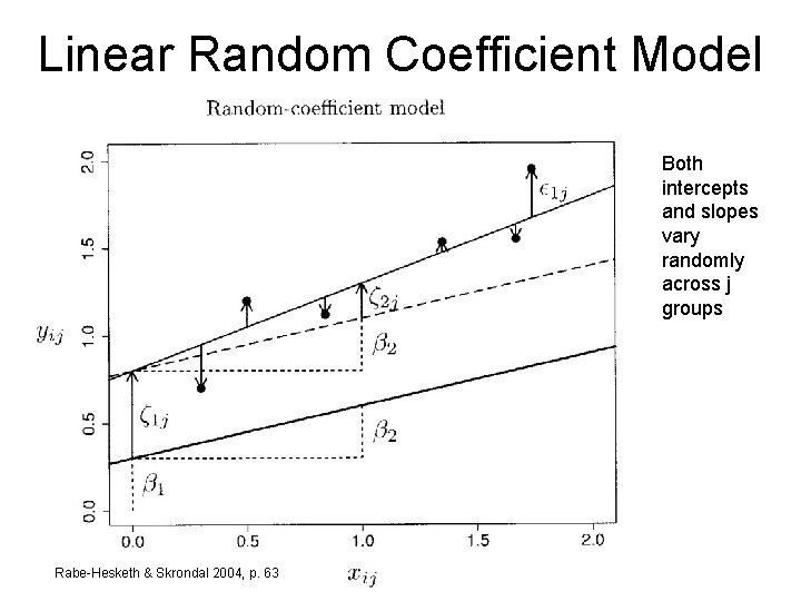
Linear Random Coefficient Model Both intercepts and slopes vary randomly across j groups Rabe-Hesketh & Skrondal 2004, p. 63

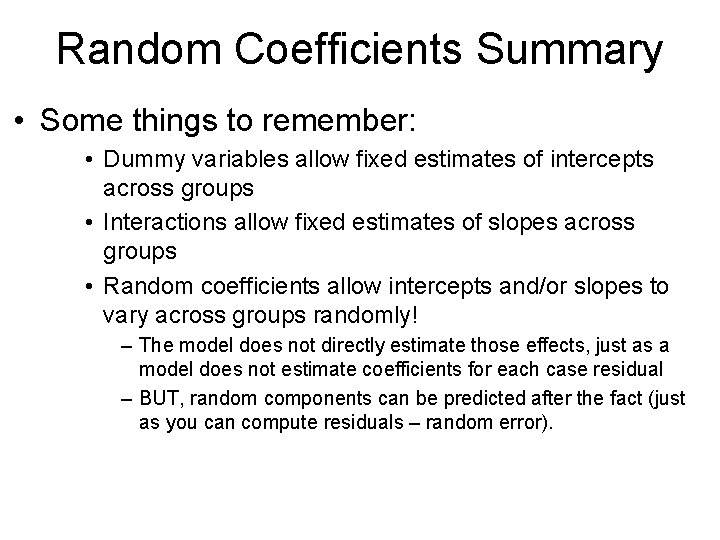
Random Coefficients Summary • Some things to remember: • Dummy variables allow fixed estimates of intercepts across groups • Interactions allow fixed estimates of slopes across groups • Random coefficients allow intercepts and/or slopes to vary across groups randomly! – The model does not directly estimate those effects, just as a model does not estimate coefficients for each case residual – BUT, random components can be predicted after the fact (just as you can compute residuals – random error).

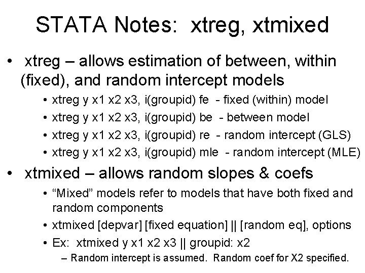
STATA Notes: xtreg, xtmixed • xtreg – allows estimation of between, within (fixed), and random intercept models • • xtreg y x 1 x 2 x 3, i(groupid) fe - fixed (within) model xtreg y x 1 x 2 x 3, i(groupid) be - between model xtreg y x 1 x 2 x 3, i(groupid) re - random intercept (GLS) xtreg y x 1 x 2 x 3, i(groupid) mle - random intercept (MLE) • xtmixed – allows random slopes & coefs • “Mixed” models refer to models that have both fixed and random components • xtmixed [depvar] [fixed equation] || [random eq], options • Ex: xtmixed y x 1 x 2 x 3 || groupid: x 2 – Random intercept is assumed. Random coef for X 2 specified.

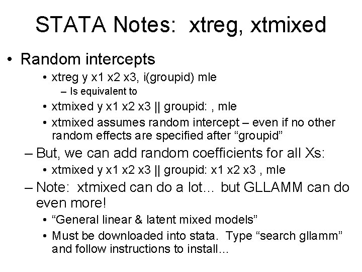
STATA Notes: xtreg, xtmixed • Random intercepts • xtreg y x 1 x 2 x 3, i(groupid) mle – Is equivalent to • xtmixed y x 1 x 2 x 3 || groupid: , mle • xtmixed assumes random intercept – even if no other random effects are specified after “groupid” – But, we can add random coefficients for all Xs: • xtmixed y x 1 x 2 x 3 || groupid: x 1 x 2 x 3 , mle – Note: xtmixed can do a lot… but GLLAMM can do even more! • “General linear & latent mixed models” • Must be downloaded into stata. Type “search gllamm” and follow instructions to install…

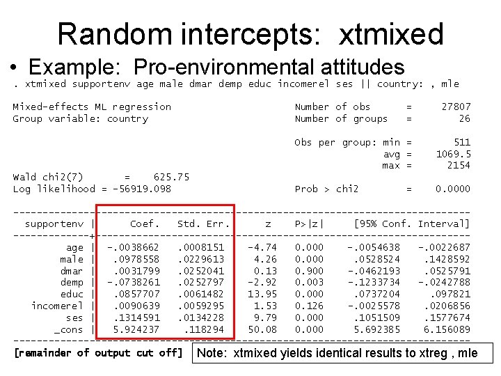
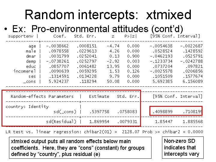
Random intercepts: xtmixed • Example: Pro-environmental attitudes. xtmixed supportenv age male dmar demp educ incomerel ses || country: , mle Mixed-effects ML regression Group variable: country Wald chi 2(7) = 625. 75 Log likelihood = -56919. 098 Number of obs Number of groups = = 27807 26 Obs per group: min = avg = max = 511 1069. 5 2154 Prob > chi 2 0. 0000 = ---------------------------------------supportenv | Coef. Std. Err. z P>|z| [95% Conf. Interval] -------+--------------------------------age | -. 0038662. 0008151 -4. 74 0. 000 -. 0054638 -. 0022687 male |. 0978558. 0229613 4. 26 0. 000. 0528524. 1428592 dmar |. 0031799. 0252041 0. 13 0. 900 -. 0462193. 0525791 demp | -. 0738261. 0252797 -2. 92 0. 003 -. 1233734 -. 0242788 educ |. 0857707. 0061482 13. 95 0. 000. 0737204. 097821 incomerel |. 0090639. 0059295 1. 53 0. 126 -. 0025578. 0206856 ses |. 1314591. 0134228 9. 79 0. 000. 1051509. 1577674 _cons | 5. 924237. 118294 50. 08 0. 000 5. 692385 6. 156089 ---------------------------------------[remainder of output cut off] Note: xtmixed yields identical results to xtreg , mle

Random intercepts: xtmixed • Ex: Pro-environmental attitudes (cont’d) supportenv | Coef. Std. Err. z P>|z| [95% Conf. Interval] -------+--------------------------------age | -. 0038662. 0008151 -4. 74 0. 000 -. 0054638 -. 0022687 male |. 0978558. 0229613 4. 26 0. 000. 0528524. 1428592 dmar |. 0031799. 0252041 0. 13 0. 900 -. 0462193. 0525791 demp | -. 0738261. 0252797 -2. 92 0. 003 -. 1233734 -. 0242788 educ |. 0857707. 0061482 13. 95 0. 000. 0737204. 097821 incomerel |. 0090639. 0059295 1. 53 0. 126 -. 0025578. 0206856 ses |. 1314591. 0134228 9. 79 0. 000. 1051509. 1577674 _cons | 5. 924237. 118294 50. 08 0. 000 5. 692385 6. 156089 -----------------------------------------------------------------------------Random-effects Parameters | Estimate Std. Err. [95% Conf. Interval] ---------------+------------------------country: Identity | sd(_cons) |. 5397758. 0758083. 4098899. 7108199 ---------------+------------------------sd(Residual) | 1. 869954. 0079331 1. 85447 1. 885568 ---------------------------------------LR test vs. linear regression: chibar 2(01) = 2128. 07 Prob >= chibar 2 = 0. 0000 xtmixed output puts all random effects below main coefficients. Here, they are “cons” (constant) for groups defined by “country”, plus residual (e) Non-zero SD indicates that intercepts vary

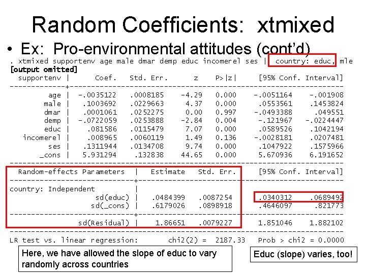
Random Coefficients: xtmixed • Ex: Pro-environmental attitudes (cont’d). xtmixed supportenv age male dmar demp educ incomerel ses || country: educ, mle [output omitted] supportenv | Coef. Std. Err. z P>|z| [95% Conf. Interval] -------+--------------------------------age | -. 0035122. 0008185 -4. 29 0. 000 -. 0051164 -. 001908 male |. 1003692. 0229663 4. 37 0. 000. 0553561. 1453824 dmar |. 0001061. 0252275 0. 00 0. 997 -. 0493388. 049551 demp | -. 0722059. 0253888 -2. 84 0. 004 -. 121967 -. 0224447 educ |. 081586. 0115479 7. 07 0. 000. 0589526. 1042194 incomerel |. 008965. 0060119 1. 49 0. 136 -. 0028181. 0207481 ses |. 1311944. 0134708 9. 74 0. 000. 1047922. 1575966 _cons | 5. 931294. 132838 44. 65 0. 000 5. 670936 6. 191652 ---------------------------------------Random-effects Parameters | Estimate Std. Err. [95% Conf. Interval] ---------------+------------------------country: Independent | sd(educ) |. 0484399. 0087254. 0340312. 0689492 sd(_cons) |. 6179026. 0898918. 4646097. 821773 ---------------+------------------------sd(Residual) | 1. 86651. 0079227 1. 851046 1. 882102 ---------------------------------------LR test vs. linear regression: chi 2(2) = 2187. 33 Prob > chi 2 = 0. 0000 Here, we have allowed the slope of educ to vary randomly across countries Educ (slope) varies, too!

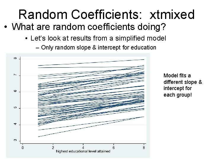
Random Coefficients: xtmixed • What are random coefficients doing? • Let’s look at results from a simplified model – Only random slope & intercept for education Model fits a different slope & intercept for each group!

Random Coefficients • Why bother with random coefficients? • 1. A solution for clustering (non-independence) – Usually people just use random intercepts, but slopes may be an issue also • 2. You can create a better-fitting model – If slopes & intercepts vary, a random coefficient model may fit better – Assuming distributional assumptions are met – Model fit compared to OLS can be tested…. • 3. Better predictions – Attention to group-specific random effects can yield better predictions (e. g. , slopes) for each group » Rather than just looking at “average” slope for all groups • 4. Helps us think about multilevel data » Ex: cross-level interactions (we’ll discuss soon!)

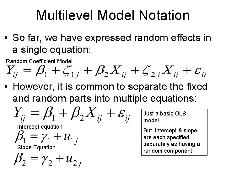
Multilevel Model Notation • So far, we have expressed random effects in a single equation: Random Coefficient Model • However, it is common to separate the fixed and random parts into multiple equations: Just a basic OLS model… Intercept equation Slope Equation But, intercept & slope are each specified separately as having a random component

Multilevel Model Notation • The “separate equation” formulation is no different from what we did before… • But it is a vivid & clear way to present your models • All random components are obvious because they are stated in separate equations • NOTE: Some software (e. g. , HLM) requires this – Rules: • 1. Specify an OLS model, just like normal • 2. Consider which OLS coefficients should have a random component – These could be the intercept or any X variable (slope) • 3. Specify an additional formula for each random coefficient.