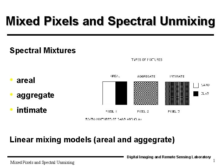
Mixed Pixels and Spectral Unmixing Spectral Mixtures areal

Mixed Pixels and Spectral Unmixing Spectral Mixtures • • • areal aggregate intimate Linear mixing models (areal and aggegrate) Digital Imaging and Remote Sensing Laboratory Mixed Pixels and Spectral Unmixing 1

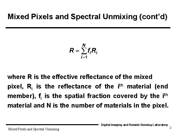
Mixed Pixels and Spectral Unmixing (cont’d) where R is the effective reflectance of the mixed pixel, Ri is the reflectance of the ith material (end member), fi is the spatial fraction covered by the ith material and N is the number of materials in the pixel. Digital Imaging and Remote Sensing Laboratory Mixed Pixels and Spectral Unmixing 2

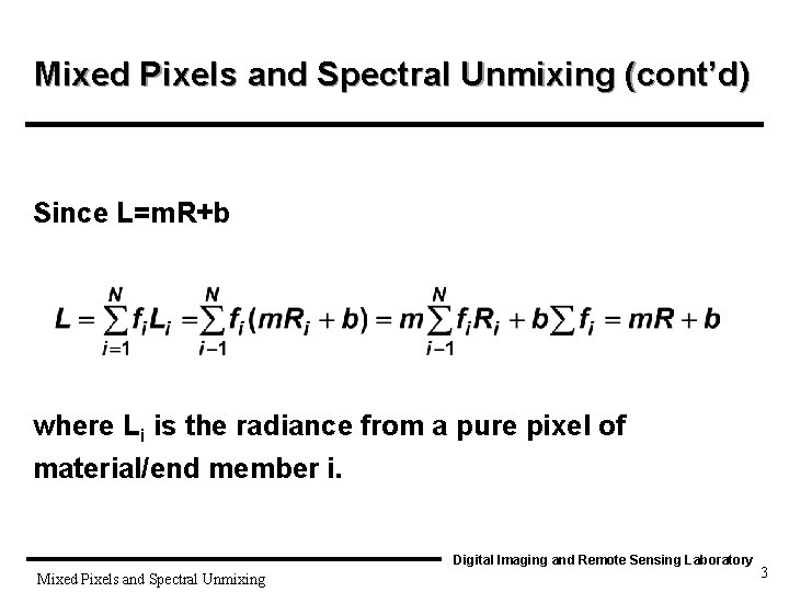
Mixed Pixels and Spectral Unmixing (cont’d) Since L=m. R+b where Li is the radiance from a pure pixel of material/end member i. Digital Imaging and Remote Sensing Laboratory Mixed Pixels and Spectral Unmixing 3

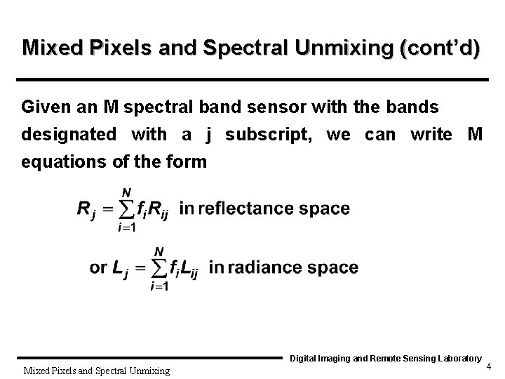
Mixed Pixels and Spectral Unmixing (cont’d) Given an M spectral band sensor with the bands designated with a j subscript, we can write M equations of the form Digital Imaging and Remote Sensing Laboratory Mixed Pixels and Spectral Unmixing 4

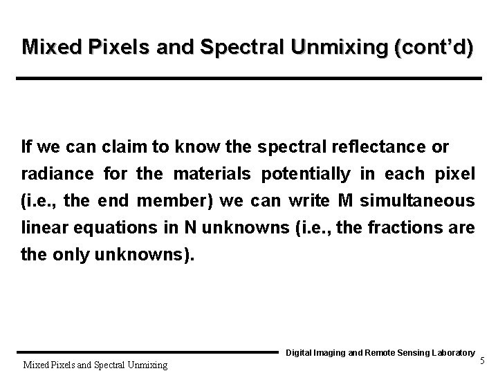
Mixed Pixels and Spectral Unmixing (cont’d) If we can claim to know the spectral reflectance or radiance for the materials potentially in each pixel (i. e. , the end member) we can write M simultaneous linear equations in N unknowns (i. e. , the fractions are the only unknowns). Digital Imaging and Remote Sensing Laboratory Mixed Pixels and Spectral Unmixing 5

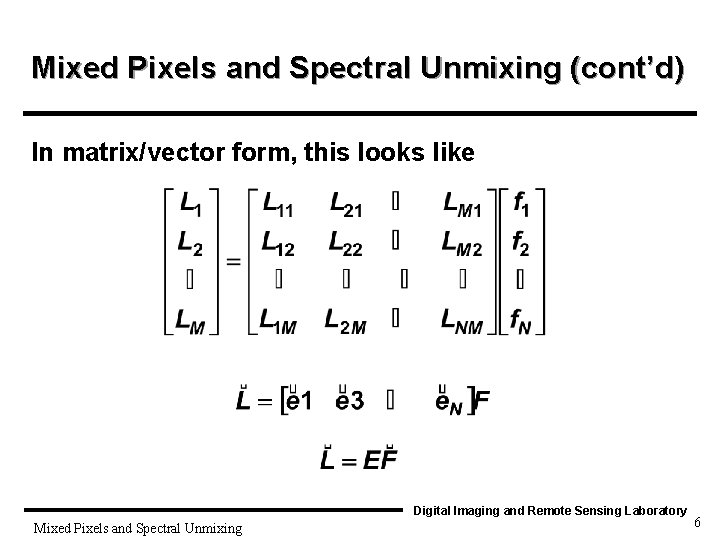
Mixed Pixels and Spectral Unmixing (cont’d) In matrix/vector form, this looks like Digital Imaging and Remote Sensing Laboratory Mixed Pixels and Spectral Unmixing 6

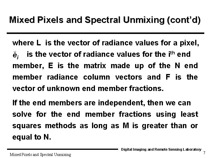
Mixed Pixels and Spectral Unmixing (cont’d) where L is the vector of radiance values for a pixel, is the vector of radiance values for the ith end member, E is the matrix made up of the N end member radiance column vectors and F is the vector of unknown end member fractions. If the end members are independent, then we can solve for the end member fractions using least squares methods as long as M is greater than or equal to N. Digital Imaging and Remote Sensing Laboratory Mixed Pixels and Spectral Unmixing 7

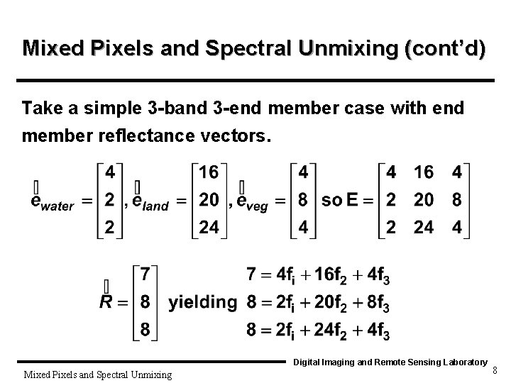
Mixed Pixels and Spectral Unmixing (cont’d) Take a simple 3 -band 3 -end member case with end member reflectance vectors. Digital Imaging and Remote Sensing Laboratory Mixed Pixels and Spectral Unmixing 8

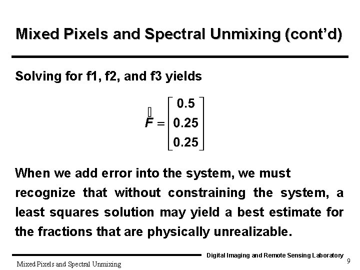
Mixed Pixels and Spectral Unmixing (cont’d) Solving for f 1, f 2, and f 3 yields When we add error into the system, we must recognize that without constraining the system, a least squares solution may yield a best estimate for the fractions that are physically unrealizable. Digital Imaging and Remote Sensing Laboratory Mixed Pixels and Spectral Unmixing 9

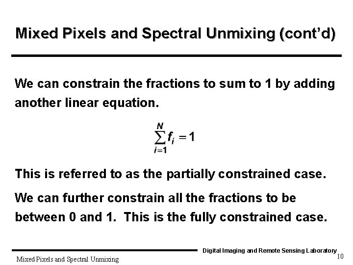
Mixed Pixels and Spectral Unmixing (cont’d) We can constrain the fractions to sum to 1 by adding another linear equation. This is referred to as the partially constrained case. We can further constrain all the fractions to be between 0 and 1. This is the fully constrained case. Digital Imaging and Remote Sensing Laboratory Mixed Pixels and Spectral Unmixing 10

Mixed Pixels and Spectral Unmixing (cont’d) Both these cases can be solved using extensions to the least squares (Robinson, 1997 and Gross, 1996). theory Digital Imaging and Remote Sensing Laboratory Mixed Pixels and Spectral Unmixing 11

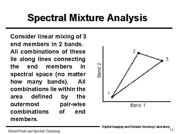
Spectral Mixture Analysis Consider linear mixing of 3 end members in 2 bands. All combinations of these lie along lines connecting the end members in spectral space (no matter how many bands). All combinations lie within the area defined by the outermost pair-wise combinations of end members. Digital Imaging and Remote Sensing Laboratory Mixed Pixels and Spectral Unmixing 12

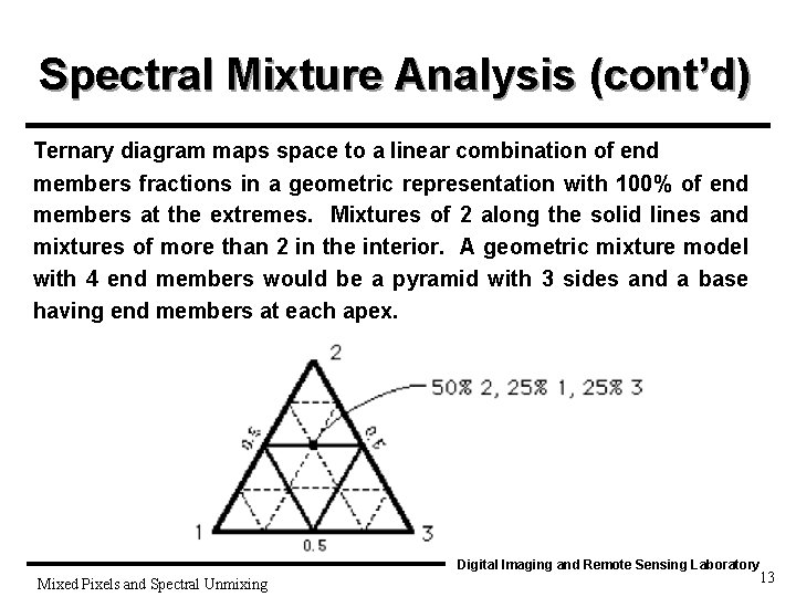
Spectral Mixture Analysis (cont’d) Ternary diagram maps space to a linear combination of end members fractions in a geometric representation with 100% of end members at the extremes. Mixtures of 2 along the solid lines and mixtures of more than 2 in the interior. A geometric mixture model with 4 end members would be a pyramid with 3 sides and a base having end members at each apex. Digital Imaging and Remote Sensing Laboratory Mixed Pixels and Spectral Unmixing 13

Mixed Pixels and Spectral Unmixing (cont’d) • Graphical illustration of mixing models • The nature of mixing suggests that all combinations of end members must lie inside of a convex hull made up of the end members Digital Imaging and Remote Sensing Laboratory Mixed Pixels and Spectral Unmixing 14

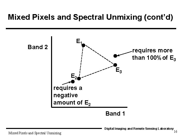
Mixed Pixels and Spectral Unmixing (cont’d) • end member concepts • The end members are assumed to be spectral extrema representing spectrally idealized examples of a land cover type. • End members greater that 1 and less that zero Digital Imaging and Remote Sensing Laboratory Mixed Pixels and Spectral Unmixing 15

Mixed Pixels and Spectral Unmixing (cont’d) E 1 Band 2 requires more than 100%of E 3 E 2 E 3 requires a negative amount of E 2 Band 1 Digital Imaging and Remote Sensing Laboratory Mixed Pixels and Spectral Unmixing 16

Mixed Pixels and Spectral Unmixing (cont’d) In order to account for brightness variations due to solar illumination effects and mixed pixels containing shadows, a shadow end member may be introduced. The shadow end member typically is assigned the spectral reflectance expected from a dark shadow element. Digital Imaging and Remote Sensing Laboratory Mixed Pixels and Spectral Unmixing 17

Mixed Pixels and Spectral Unmixing (cont’d) In general, to avoid over-fitting the end member model, a smaller number of end members is preferred. Adding more end members to the model will always reduce the residual error, but often we are just trying to fit information to the noise. Digital Imaging and Remote Sensing Laboratory Mixed Pixels and Spectral Unmixing 18

Mixed Pixels and Spectral Unmixing (cont’d) Because we may not have “pure” end members (i. e. , true extremes), it is often physically reasonable to have fractions slightly less than zero or greater than one. For this reason, the partially constrained model is often most appropriate. Digital Imaging and Remote Sensing Laboratory Mixed Pixels and Spectral Unmixing 19

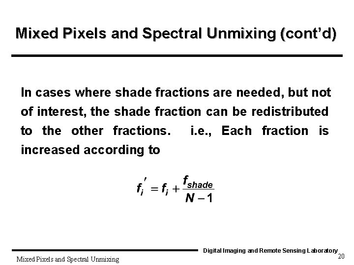
Mixed Pixels and Spectral Unmixing (cont’d) In cases where shade fractions are needed, but not of interest, the shade fraction can be redistributed to the other fractions. i. e. , Each fraction is increased according to Digital Imaging and Remote Sensing Laboratory Mixed Pixels and Spectral Unmixing 20

Mixed Pixels and Spectral Unmixing (cont’d) • • • Image. Fractions maps. End member selection and model generation. Digital Imaging and Remote Sensing Laboratory Mixed Pixels and Spectral Unmixing 21

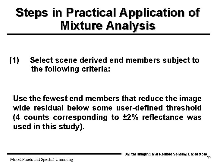
Steps in Practical Application of Mixture Analysis (1) Select scene derived end members subject to the following criteria: Use the fewest end members that reduce the image wide residual below some user-defined threshold (4 counts corresponding to ± 2% reflectance was used in this study). Digital Imaging and Remote Sensing Laboratory Mixed Pixels and Spectral Unmixing 22

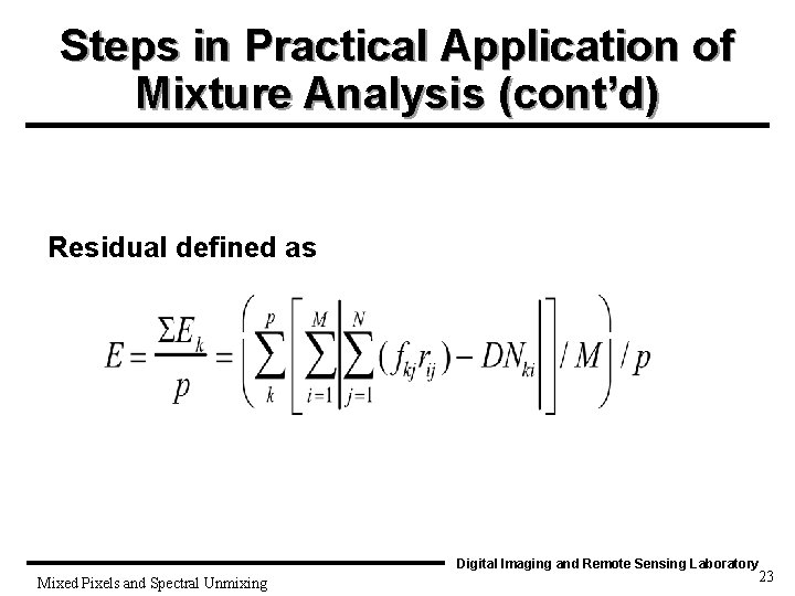
Steps in Practical Application of Mixture Analysis (cont’d) Residual defined as Digital Imaging and Remote Sensing Laboratory Mixed Pixels and Spectral Unmixing 23

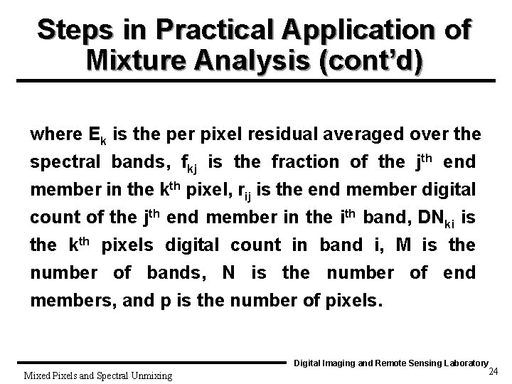
Steps in Practical Application of Mixture Analysis (cont’d) where Ek is the per pixel residual averaged over the spectral bands, fkj is the fraction of the jth end member in the kth pixel, rij is the end member digital count of the jth end member in the ith band, DNki is the kth pixels digital count in band i, M is the number of bands, N is the number of end members, and p is the number of pixels. Digital Imaging and Remote Sensing Laboratory Mixed Pixels and Spectral Unmixing 24

Steps in Practical Application of Mixture Analysis (cont’d) In practice, the user smartly picks image derived end members, including shade, in order of decreasing spectral contrast. (i. e. , High contrast end members with respect to shade added first. ) Adding end members until E is below the threshold value. Digital Imaging and Remote Sensing Laboratory Mixed Pixels and Spectral Unmixing 25

Steps in Practical Application of Mixture Analysis (cont’d) End members can be picked by taking pixels and sequentially testing to see if they are linear combinations of each other (thresholded to some criteria). As each new pixel is tested, it is either a combination or a new end member. New end members can cause previous ones to be replaced. Usually this is not done image wide, but rather the user introduces candidate end members. Brightly lit (low shade) samples should be selected. Digital Imaging and Remote Sensing Laboratory Mixed Pixels and Spectral Unmixing 26

Steps in Practical Application of Mixture Analysis (cont’d) End members may also be simply defined by context if the user is familiar with the site. Note image derived end members may be (and usually are) mixtures themselves. The shade end member accounts for illumination effects (cos ), shape factor (F), shadowing, and any other source of mean level brightness change. Digital Imaging and Remote Sensing Laboratory Mixed Pixels and Spectral Unmixing 27

Steps in Practical Application of Mixture Analysis (cont’d) The shade end member can be selected from pixels in shadow if resolvable. Sometimes a dark object can be selected as an estimate, or atmosphere and sensor calibration can be used to estimate the signal expected from a shadow ( 0% reflective). Digital Imaging and Remote Sensing Laboratory Mixed Pixels and Spectral Unmixing 28

Steps in Practical Application of Mixture Analysis (cont’d) Next the image end members can be modeled as mixtures of laboratory spectra and the calibration coefficients determined. We can test end members by (1) image wide residual error (Equation 4 or an RMS equivalent) testing both magnitude and spatial pattern, by (2) fraction continuity - context (i. e. , do the fraction maps make intuitive sense? ). Included in this is a mapping of [1 Fshade] scaled as brightness which should mimic to topography. Digital Imaging and Remote Sensing Laboratory Mixed Pixels and Spectral Unmixing 29

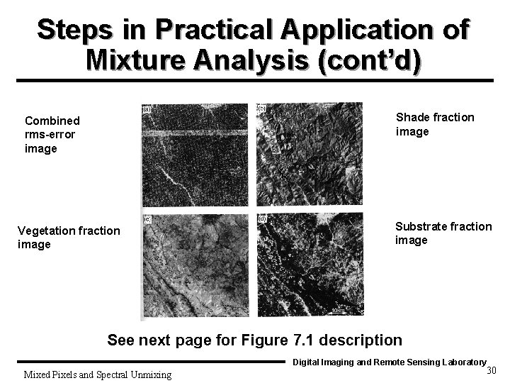
Steps in Practical Application of Mixture Analysis (cont’d) Shade fraction image Combined rms-error image Vegetation fraction image Substrate fraction image See next page for Figure 7. 1 description Digital Imaging and Remote Sensing Laboratory Mixed Pixels and Spectral Unmixing 30

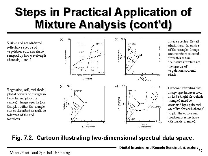
Steps in Practical Application of Mixture Analysis (cont’d) (3) If fraction maps are scaled for display as DC=(fi+1)· 100, then the normal range will be 100 -200 and out of range values (negative and greater than one) can be identified. Note these values can regularly occur in the partially constrained case and either indicate the lack of purity of an end member or failure to include an end member. These out of range values can be color coded to flag out of range values in the fraction maps giving us a trend criteria for the quality of the end member selection. See Figure 7. 2. Digital Imaging and Remote Sensing Laboratory Mixed Pixels and Spectral Unmixing 31

Steps in Practical Application of Mixture Analysis (cont’d) Visible and near-infrared reflectance spectra of vegetation, soil, and shade sampled by two wavelength channels, 1 and 2. Image spectra (Xs) all cluster near the center of the triangle. Image end members selected from this set are themselves mixtures of the spectra of vegetation, soil and shade Vegetation, soil, and shade plot at corners of triangle in two-channel plot (open circles). Image spectra (Xs) that plot within the triangle can be described as realistic mixtures of the end members. Cartoon illustrating that image spectra measured in DN’s (light Xs outside triangle) must be corrected by a gain and an offset for each channel to plot the equivalent position in reflectance (Xs inside triangle). Fig. 7. 2. Cartoon illustrating two-dimensional spectral data space. Digital Imaging and Remote Sensing Laboratory Mixed Pixels and Spectral Unmixing 32

Linked Models Rather than try to unmix a complex image simultaneous with many possible end members, it is often desirable to unmix on a smaller number of end members in a localized region and then link the solutions together. We can use masks to avoid unmixing the same area in two ways. Digital Imaging and Remote Sensing Laboratory Mixed Pixels and Spectral Unmixing 33

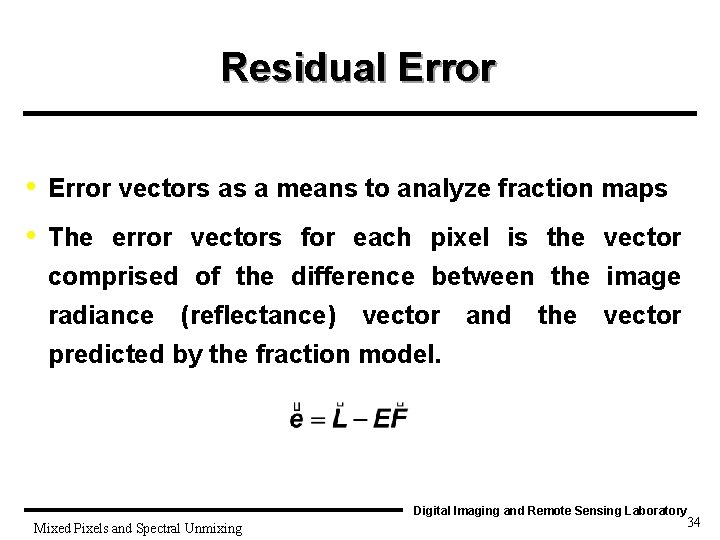
Residual Error • • Error vectors as a means to analyze fraction maps The error vectors for each pixel is the vector comprised of the difference between the image radiance (reflectance) vector and predicted by the fraction model. the vector Digital Imaging and Remote Sensing Laboratory Mixed Pixels and Spectral Unmixing 34

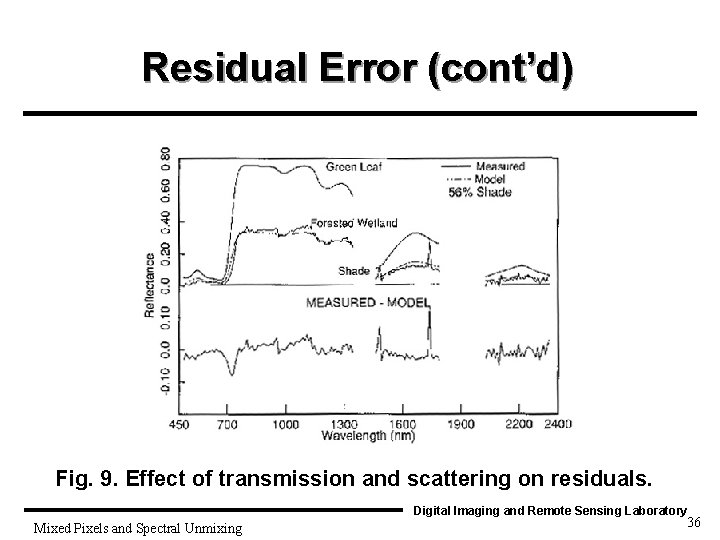
Residual Error (cont’d) • We can make a map of the magnitude of the errors as an indication of locations where the model is inadequate • We can also look at the spectral shape of the error and compare it to spectral features of interest. Digital Imaging and Remote Sensing Laboratory Mixed Pixels and Spectral Unmixing 35

Residual Error (cont’d) Fig. 9. Effect of transmission and scattering on residuals. Digital Imaging and Remote Sensing Laboratory Mixed Pixels and Spectral Unmixing 36

Residual Error (cont’d) • If we have a target material(s) representing a small number of pixels, it may be more effective to leave it out of the end member analysis and just look closely at the error vectors. • We may map an error spectrally localized to characteristic features in the target material. Digital Imaging and Remote Sensing Laboratory Mixed Pixels and Spectral Unmixing 37

Residual Error (cont’d) • What is an end member and what use are end member maps. – Fraction maps – Associations as end members – Combining fractions to form associations – Class maps with transition classes Digital Imaging and Remote Sensing Laboratory Mixed Pixels and Spectral Unmixing 38

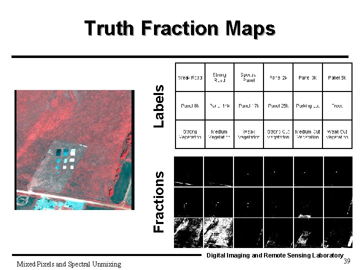
Fractions Labels Truth Fraction Maps Digital Imaging and Remote Sensing Laboratory Mixed Pixels and Spectral Unmixing 39

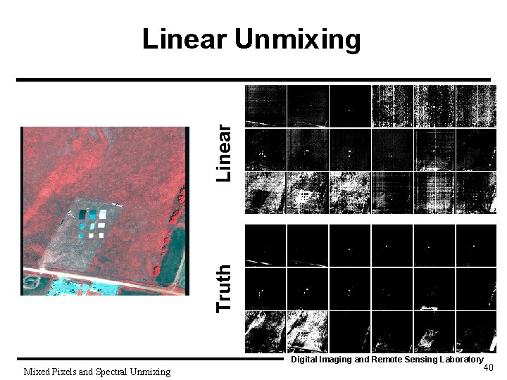
Truth Linear Unmixing Digital Imaging and Remote Sensing Laboratory Mixed Pixels and Spectral Unmixing 40