Methods for Dummies Secondlevel Analysis for f MRI

Methods for Dummies Second-level Analysis (for f. MRI) Justyna Ekert & Alex Hopkins Expert: Guillaume Flandin

Overview 1. 2. 3. 4. 5. Recap of first-level analysis What is second-level analysis? Fixed versus random effects How do we analyse random effects? Practical demonstration 2

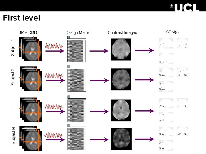
First level Subject N … Subject 2 Subject 1 f. MRI data Design Matrix Contrast Images SPM{t}

Second level analysis • Deals with groups of subjects, e. g. Patients vs. control Brain activity*trait anxiety • which voxels consistently show significant activity within our group • We would also like to be able to generalise our results to non-tested subjects 4

Overview 1. 2. 3. 4. 5. Recap of first-level analysis What is second-level analysis? Fixed versus random effects How do we analyse random effects? Practical demonstration 5

Fixed versus random effects Different assumptions about the source of random variation in voxel activity

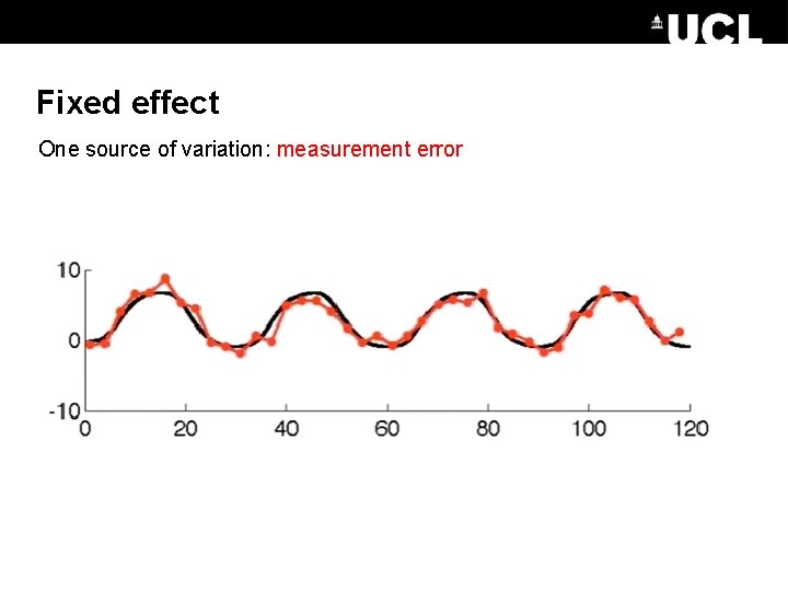
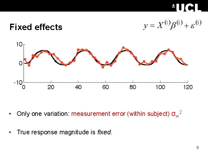
Fixed effect One source of variation: measurement error

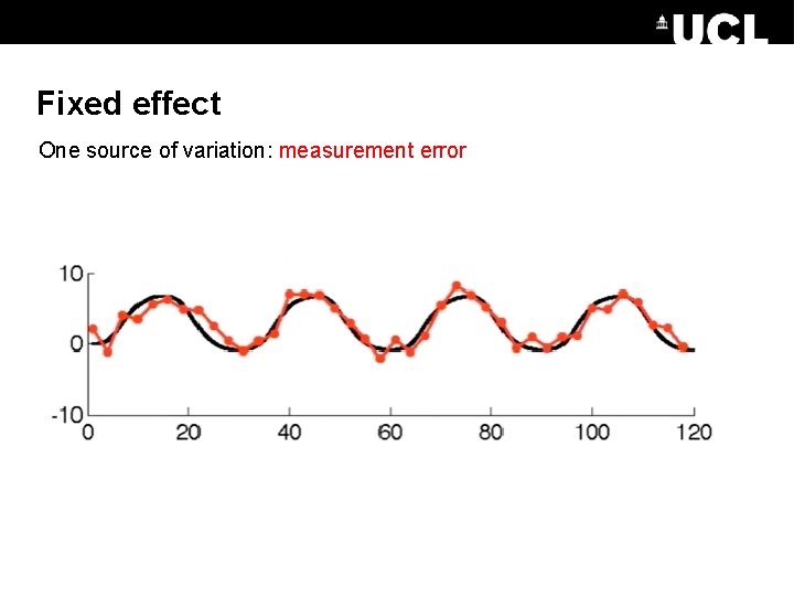
Fixed effect One source of variation: measurement error

Fixed effects • Only one variation: measurement error (within subject) σw 2 • True response magnitude is fixed. 9

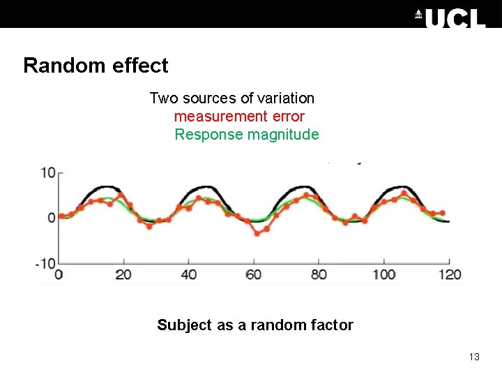
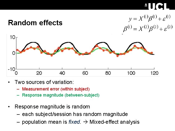
Random effects analysis (RFX) • Synonymous with ‘mixed effects models’. • Assumes our sample is a set of individuals taken at random from the population of interest. • To do this we need to consider the between subject variance, σb 2, as well as σw 2 – and estimate the likely variance of the population from which our sample is derived. 10

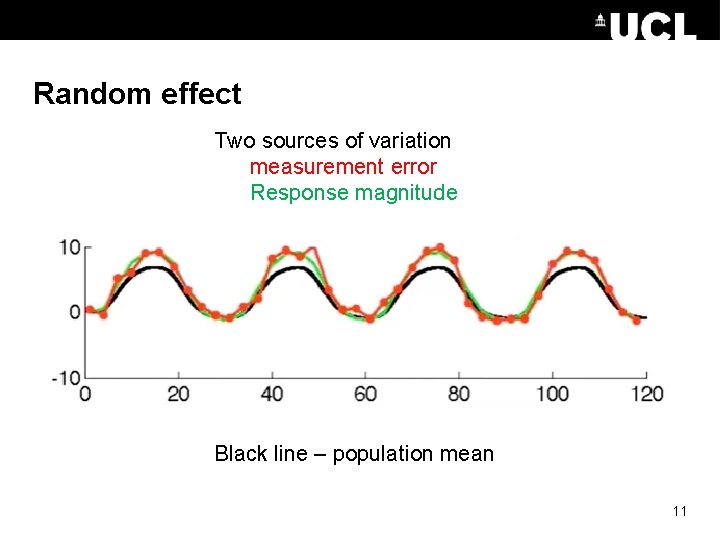
Random effect Two sources of variation measurement error Response magnitude Black line – population mean 11

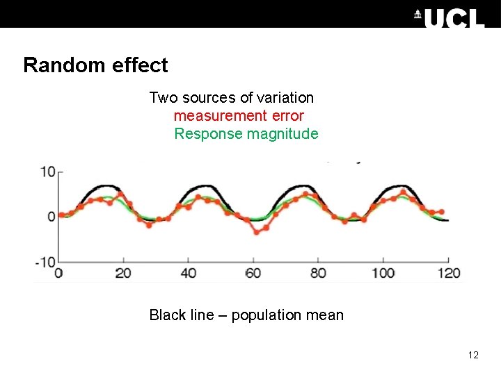
Random effect Two sources of variation measurement error Response magnitude Black line – population mean 12

Random effect Two sources of variation measurement error Response magnitude Subject as a random factor 13

Random effects • Two sources of variation: – Measurement error (within subject) – Response magnitude (between-subject) • Response magnitude is random – each subject/session has random magnitude – population mean is fixed. Mixed-effect analysis

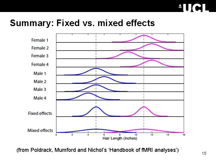
Summary: Fixed vs. mixed effects (from Poldrack, Mumford and Nichol’s ‘Handbook of f. MRI analyses’) 15

Scan more subjects! Because the between-subject variance is greater than the within subject variance, scanning time is best used in scanning more subjects rather than scanning individual subjects for longer. 16

Fixed-effects: We can only say something about our particular group of subjects No generalisation case studies Random-effects: We make inferences about the population from which the subjects were drawn generalisation possible 17

“Mixed effects models should be used whenever data are grouped within certain levels of a population and inferences are to be applied to the entire population. ” - Mumford and Poldrack (2007) 18

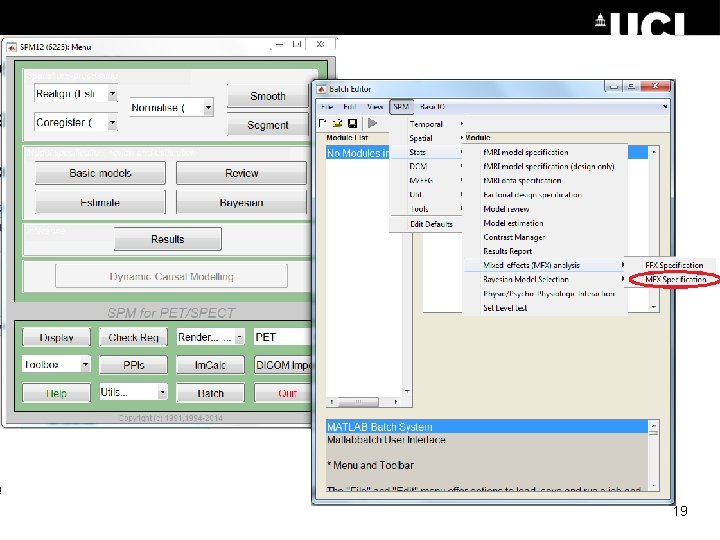
19

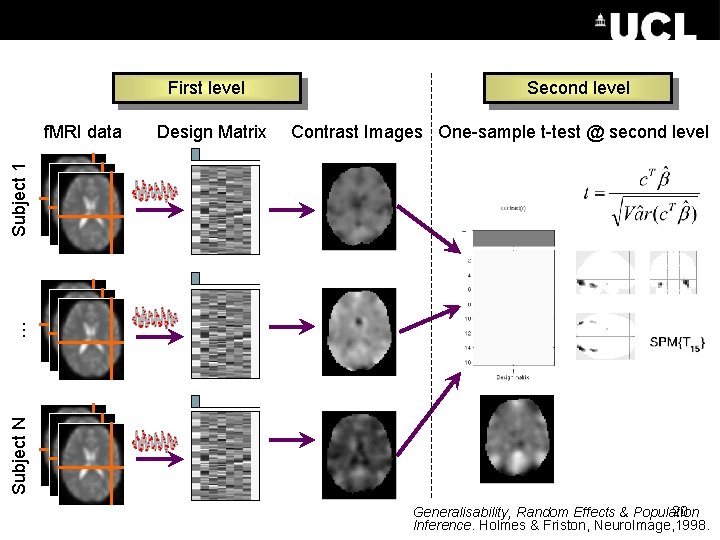
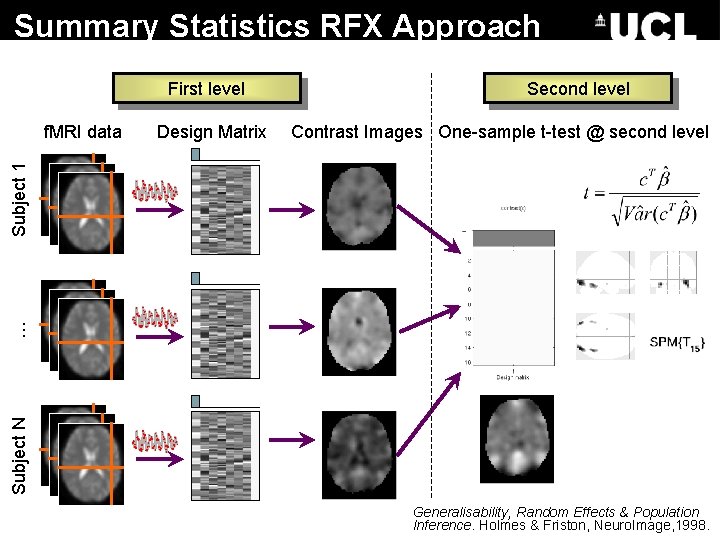
First level Design Matrix Contrast Images One-sample t-test @ second level Subject N … Subject 1 f. MRI data Second level 20 Generalisability, Random Effects & Population Inference. Holmes & Friston, Neuro. Image, 1998.

Methods for Random Effects Hierarchical • Most accurate method – gold standard • Set up a GLM containing parameters for the effects and variances at both the subject AND group levels, to all be estimated at the same time. • Estimates subject and group statistics via “iterative looping” • Computationally demanding 21

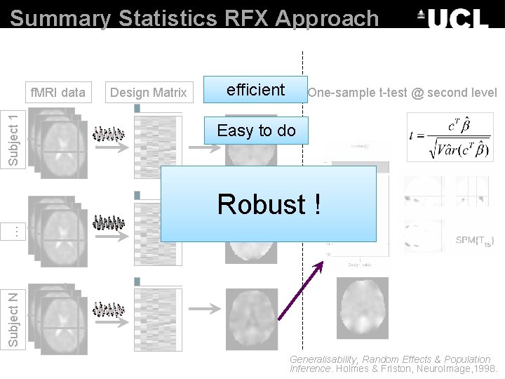
Methods for random effects Summary statistics • 1 st level design for all subjects must be the SAME • Uses the sample means as in the first level analysis • Gives exact same results as hierarchical model (when the within-subject variance is the same for all subjects) • Validity is undermined by presence of extreme outliers. 22

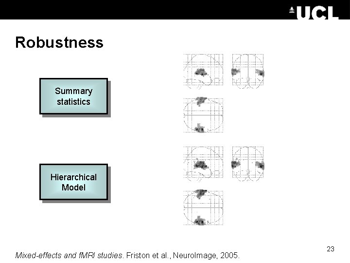
Robustness Summary statistics Hierarchical Model Mixed-effects and f. MRI studies. Friston et al. , Neuro. Image, 2005. 23

Overview 1. 2. 3. 4. 5. Recap of first-level analysis What is second-level analysis? Fixed versus random effects How do we analyse random effects? Practical demonstration 24

Summary Statistics RFX Approach First level Design Matrix Contrast Images One-sample t-test @ second level Subject N … Subject 1 f. MRI data Second level Generalisability, Random Effects & Population Inference. Holmes & Friston, Neuro. Image, 1998.

Summary Statistics RFX Approach Subject 1 f. MRI data Design Matrix efficient One-sample t-test @ second level Contrast Images Easy to do Subject N … Robust ! Generalisability, Random Effects & Population Inference. Holmes & Friston, Neuro. Image, 1998.

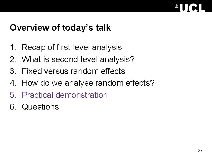
Overview of today’s talk 1. 2. 3. 4. 5. 6. Recap of first-level analysis What is second-level analysis? Fixed versus random effects How do we analyse random effects? Practical demonstration Questions 27

Buttonpressing 28

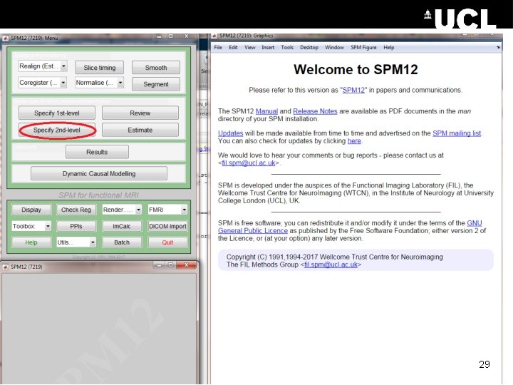
29

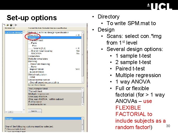
Set-up options • Directory • To write SPM. mat to • Design • Scans: select con. *img from 1 st level • Several design options: • 1 sample t-test • 2 sample t-test • Paired t-test • Multiple regression • 1 way ANOVA • Full or flexible factorial (for > 1 way ANOVAs – use FLEXIBLE FACTORIAL to include subjects as a 30 random factor!)

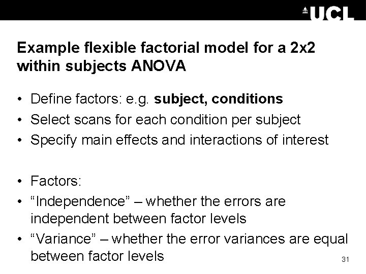
Example flexible factorial model for a 2 x 2 within subjects ANOVA • Define factors: e. g. subject, conditions • Select scans for each condition per subject • Specify main effects and interactions of interest • Factors: • “Independence” – whether the errors are independent between factor levels • “Variance” – whether the error variances are equal between factor levels 31

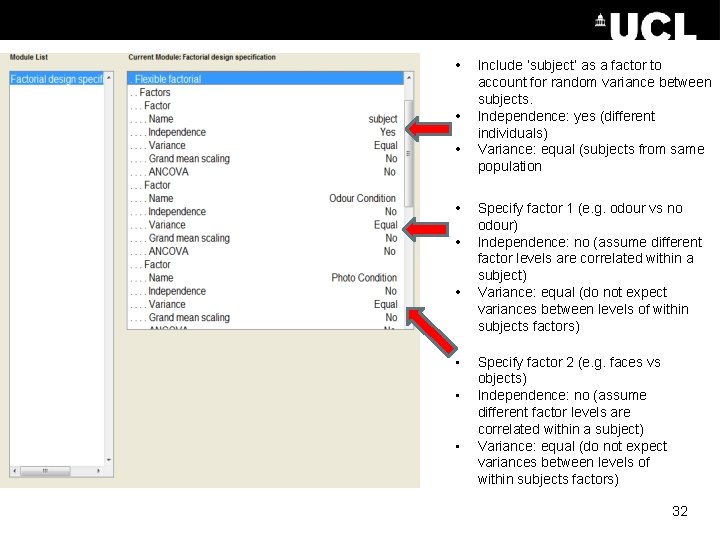
• • • Include ‘subject’ as a factor to account for random variance between subjects. Independence: yes (different individuals) Variance: equal (subjects from same population Specify factor 1 (e. g. odour vs no odour) Independence: no (assume different factor levels are correlated within a subject) Variance: equal (do not expect variances between levels of within subjects factors) Specify factor 2 (e. g. faces vs objects) Independence: no (assume different factor levels are correlated within a subject) Variance: equal (do not expect variances between levels of within subjects factors) 32

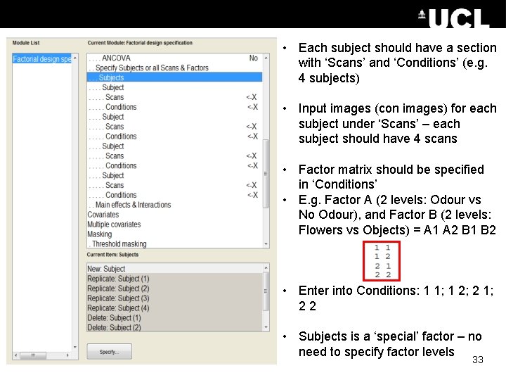
• Each subject should have a section with ‘Scans’ and ‘Conditions’ (e. g. 4 subjects) • Input images (con images) for each subject under ‘Scans’ – each subject should have 4 scans • Factor matrix should be specified in ‘Conditions’ • E. g. Factor A (2 levels: Odour vs No Odour), and Factor B (2 levels: Flowers vs Objects) = A 1 A 2 B 1 B 2 • Enter into Conditions: 1 1; 1 2; 2 1; 2 2 • Subjects is a ‘special’ factor – no need to specify factor levels 33

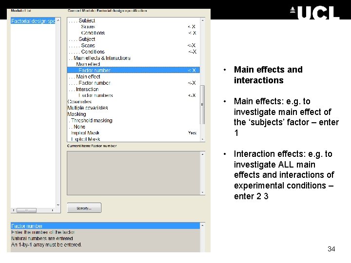
• Main effects and interactions • Main effects: e. g. to investigate main effect of the ‘subjects’ factor – enter 1 • Interaction effects: e. g. to investigate ALL main effects and interactions of experimental conditions – enter 2 3 34

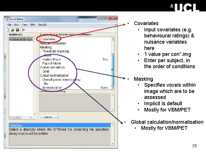
• Covariates • Input covariates (e. g. behavioural ratings) & nuisance variables here • 1 value per con*. img • Enter per subject, in the order of conditions • Masking • Specifies voxels within image which are to be assessed • Implicit is default • Mostly for VBM/PET • Global calculation/normalisation • Mostly for VBM/PET 35

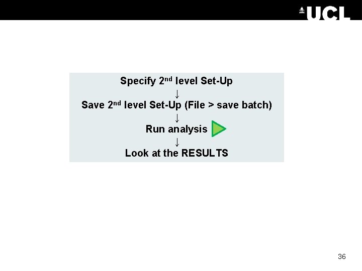
Specify 2 nd level Set-Up ↓ Save 2 nd level Set-Up (File > save batch) ↓ Run analysis ↓ Look at the RESULTS 36

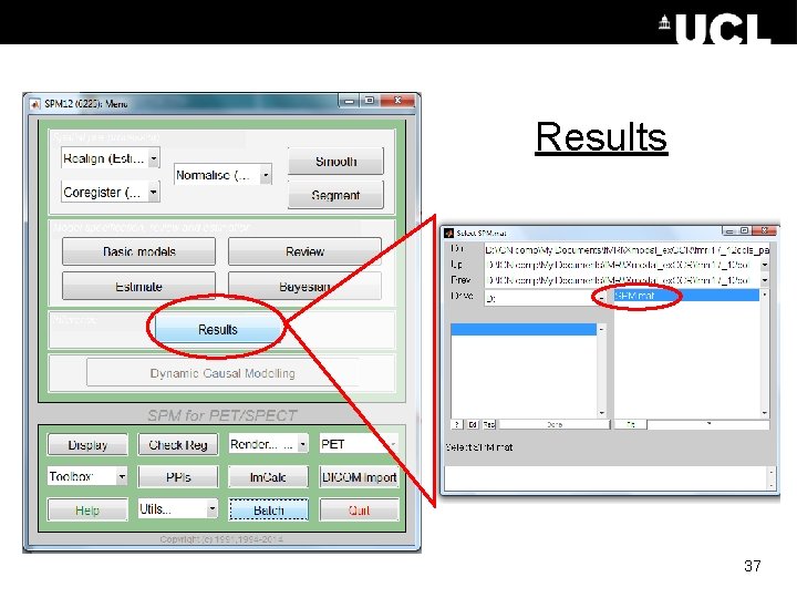
Results 37

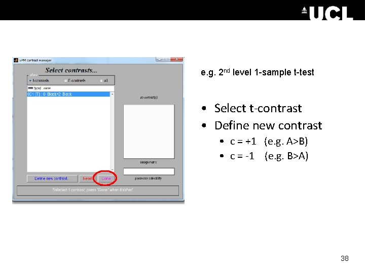
e. g. 2 nd level 1 -sample t-test • Select t-contrast • Define new contrast • c = +1 (e. g. A>B) • c = -1 (e. g. B>A) 38

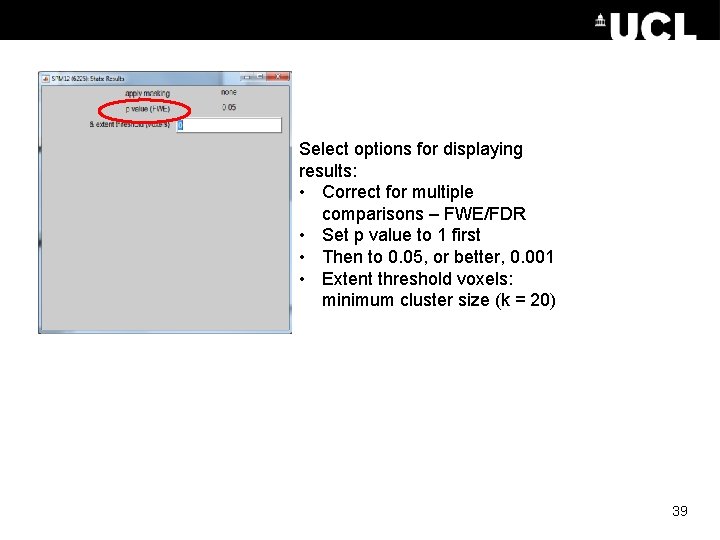
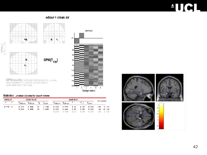
Select options for displaying results: • Correct for multiple comparisons – FWE/FDR • Set p value to 1 first • Then to 0. 05, or better, 0. 001 • Extent threshold voxels: minimum cluster size (k = 20) 39

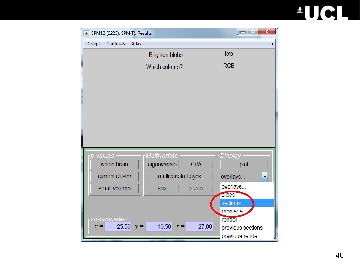
40

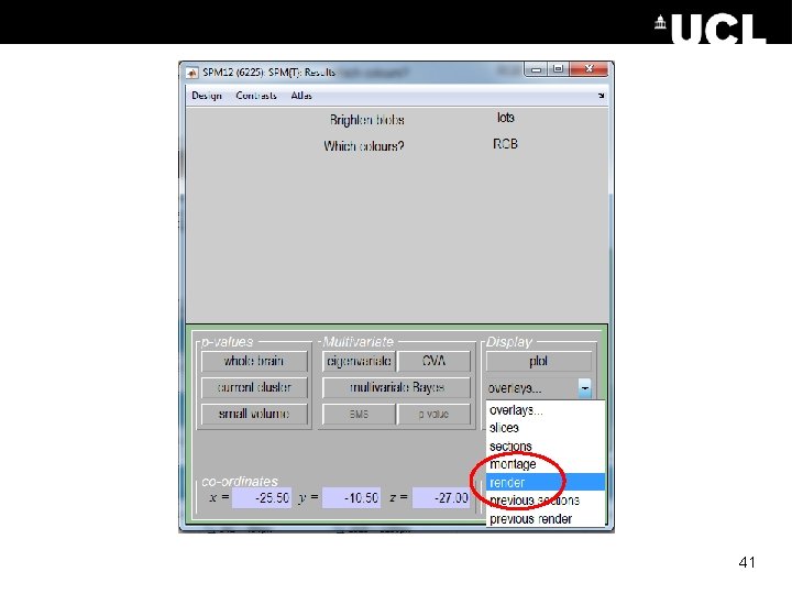
41

42

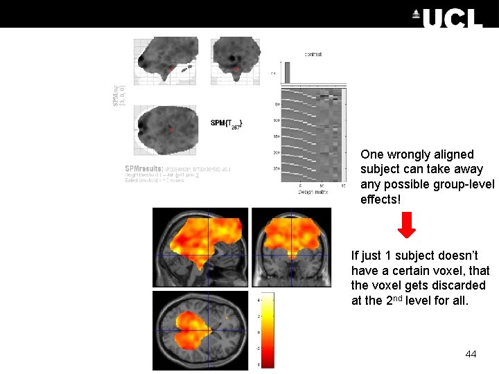
Suggestions • Always also check results at p = 1 uncorrected (you should see a full brain activation -> if not there is a problem) • If no full brain: probably one (or more) participants had a wrong realignment/normalization! 43

One wrongly aligned subject can take away any possible group-level effects! If just 1 subject doesn’t have a certain voxel, that the voxel gets discarded at the 2 nd level for all. 44

Summary • For f. MRI data, usually preferable to use RFX analysis, not FFX • Hierarchical models provide gold standard for RFX , BUT computationally intensive • Summary statistics = robust method for RFX group analysis 45

Resources • • • Previous Mf. D slides Glascher, J. & Gitelman, D. (2008) Contrast weights in flexible factorial design with multiple groups of subjects. Slides from Guillaume Flandin’s talk in Zurich, Feb 2014 Mumford, J. A. , & Poldrack, R. A. (2007). Modeling group f. MRI data. Social cognitive and affective neuroscience, 2(3), 251 -257. Friston, K. J. , Stephan, K. E. , Lund, T. E. , Morcom, A. , & Kiebel, S. (2005). Mixed-effects and f. MRI studies. Neuroimage, 24(1), 244 -252.