Methods for Dummies Second level Analysis for f

Methods for Dummies Second level Analysis (for f. MRI) Chris Hardy, Alex Fellows Expert: Guillaume Flandin

Overview of today’s talk 1. 2. 3. 4. 5. 6. Recap of first level analysis What is second level analysis? Fixed vs. random effects How do we analyse random effects? Practical demonstration Questions 2

Overview of today’s talk 1. 2. 3. 4. 5. 6. Recap of first level analysis What is second level analysis? Fixed vs. random effects How do we analyse random effects? Practical demonstration Questions 3

4

1 st Level Analysis is within subject Y f. MRI scans = X x β + ϵ Voxel time course Time (e. g. TR = 3 s) 5

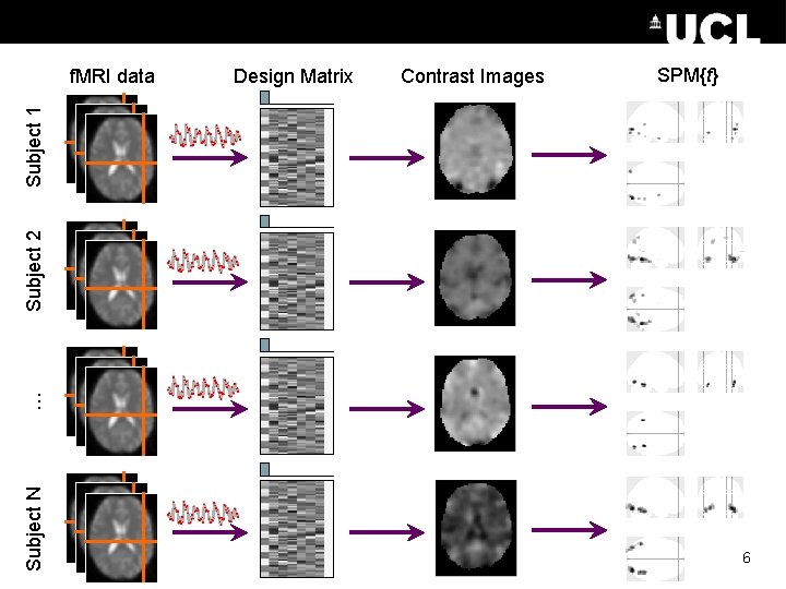
Design Matrix Contrast Images SPM{t} Subject N … Subject 2 Subject 1 f. MRI data 6

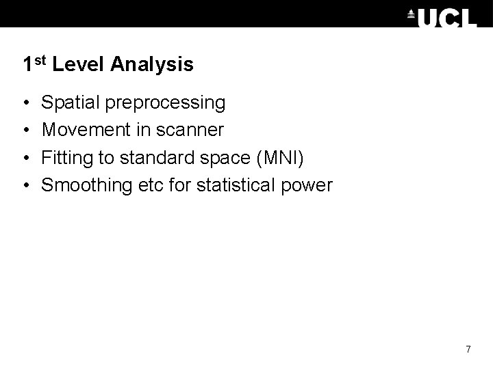
1 st Level Analysis • • Spatial preprocessing Movement in scanner Fitting to standard space (MNI) Smoothing etc for statistical power 7

Overview of today’s talk 1. 2. 3. 4. 5. 6. 7. Recap of first level analysis Second level analysis Fixed vs. random effects How do we analyse random effects? Multiple conditions Practical demonstration Questions 8

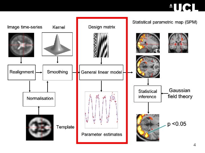
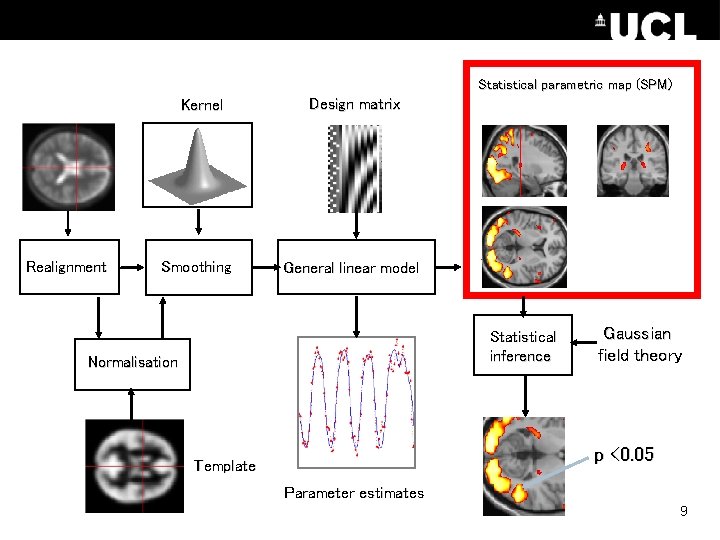
Statistical parametric map (SPM) Kernel Realignment Smoothing Design matrix General linear model Statistical inference Normalisation Gaussian field theory p <0. 05 Template Parameter estimates 9

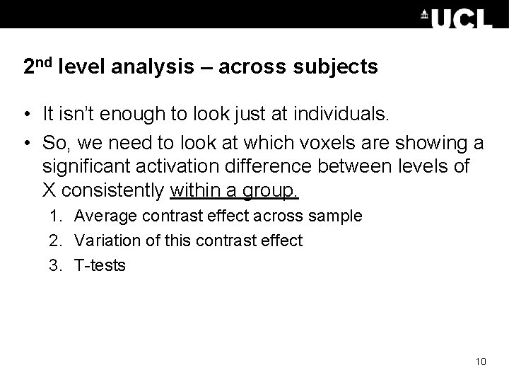
2 nd level analysis – across subjects • It isn’t enough to look just at individuals. • So, we need to look at which voxels are showing a significant activation difference between levels of X consistently within a group. 1. Average contrast effect across sample 2. Variation of this contrast effect 3. T-tests 10

Overview of today’s talk 1. 2. 3. 4. 5. 6. Recap of first level analysis What is second level analysis? Fixed vs. random effects How do we analyse random effects? Practical demonstration Questions 11

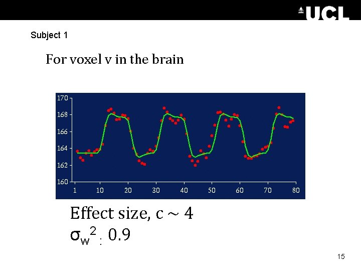
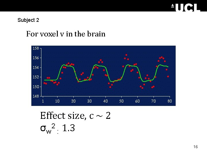
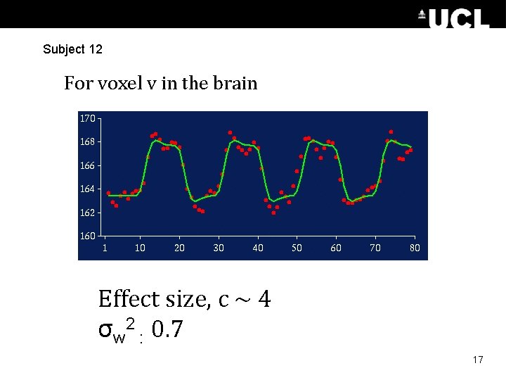
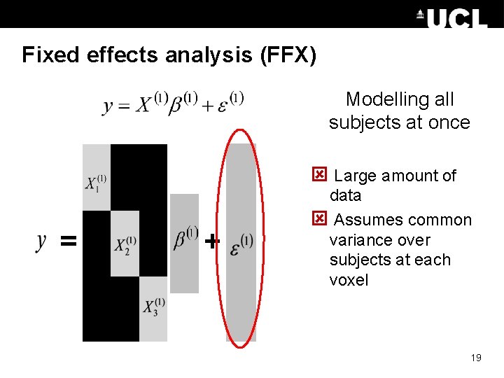
Fixed effects analysis • Each subject in an experiment repeats trials of each type many times. • The variation among the responses for each level of the design matrix (X) for a given subject gives us the within-subject variance, σw 2. • So, if we take the group effect size as the mean of responses across our subjects and analyse it with respect to σw 2. 12

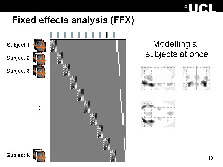
Fixed effects analysis (FFX) Modelling all subjects at once Subject 1 Subject 2 … Subject 3 Subject N 13

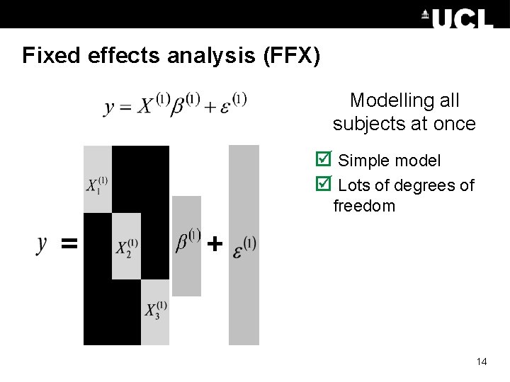
Fixed effects analysis (FFX) Modelling all subjects at once þ Simple model þ Lots of degrees of freedom = + 14

Subject 1 For voxel v in the brain Effect size, c ~ 4 σw 2 : 0. 9 15

Subject 2 For voxel v in the brain Effect size, c ~ 2 σw 2 : 1. 3 16

Subject 12 For voxel v in the brain Effect size, c ~ 4 σw 2 : 0. 7 17

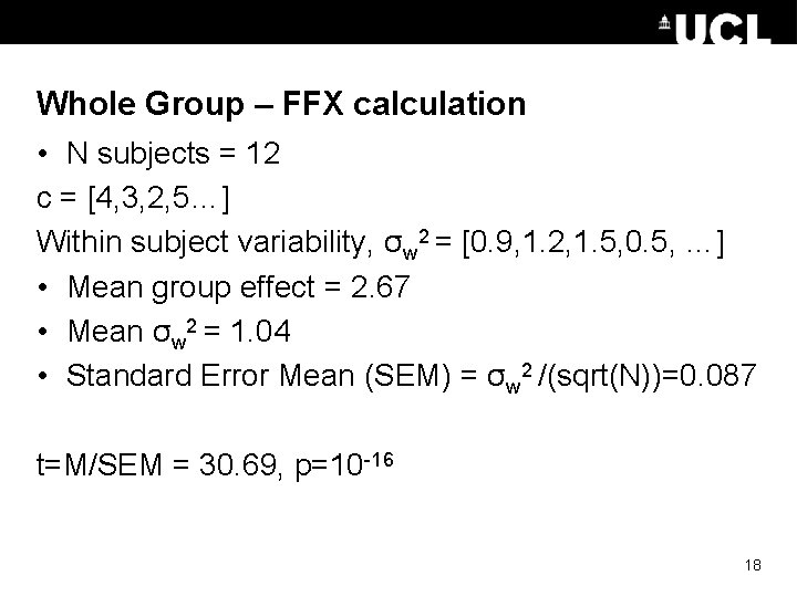
Whole Group – FFX calculation • N subjects = 12 c = [4, 3, 2, 5…] Within subject variability, σw 2 = [0. 9, 1. 2, 1. 5, 0. 5, …] • Mean group effect = 2. 67 • Mean σw 2 = 1. 04 • Standard Error Mean (SEM) = σw 2 /(sqrt(N))=0. 087 t=M/SEM = 30. 69, p=10 -16 18

Fixed effects analysis (FFX) Modelling all subjects at once ý Large amount of = + data ý Assumes common variance over subjects at each voxel 19

Random effects analysis (RFX) • Synonymous with ‘mixed effects models’. • Assumes our sample is a set of individuals taken at random from the population of interest. • To do this we need to consider the between subject variance, σb 2, as well as σw 2 – and estimate the likely variance of the population from which our sample is derived. 20

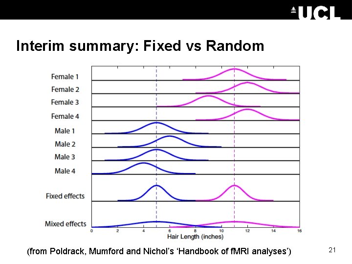
Interim summary: Fixed vs Random (from Poldrack, Mumford and Nichol’s ‘Handbook of f. MRI analyses’) 21

“Mixed effects models should be used whenever data are grouped within certain levels of a population and inferences are to be applied to the entire population. ” - Mumford and Poldrack (2007) 22

Overview of today’s talk 1. 2. 3. 4. 5. 6. Recap of first level analysis What is second level analysis? Fixed vs. random effects How do we analyse random effects? Practical demonstration Questions 23

Random effects analysis (RFX) - Methods • Hierarchical • Summary statistics approach 24

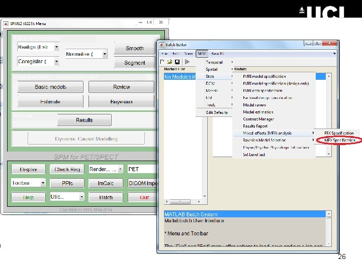
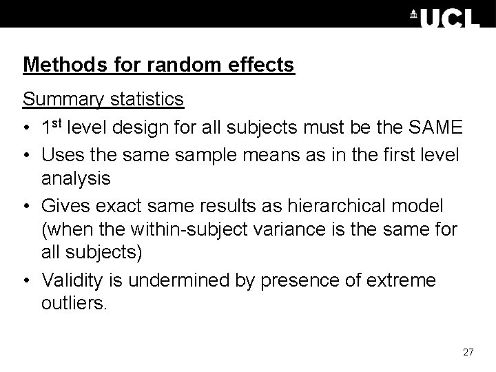
Methods for Random Effects Hierarchical • Most accurate method – gold standard • Set up a GLM containing parameters for the effects and variances at both the subject AND group levels, to all be estimated at the same time. • Estimates subject and group statistics via “iterative looping” • Computationally demanding 25

26

Methods for random effects Summary statistics • 1 st level design for all subjects must be the SAME • Uses the sample means as in the first level analysis • Gives exact same results as hierarchical model (when the within-subject variance is the same for all subjects) • Validity is undermined by presence of extreme outliers. 27

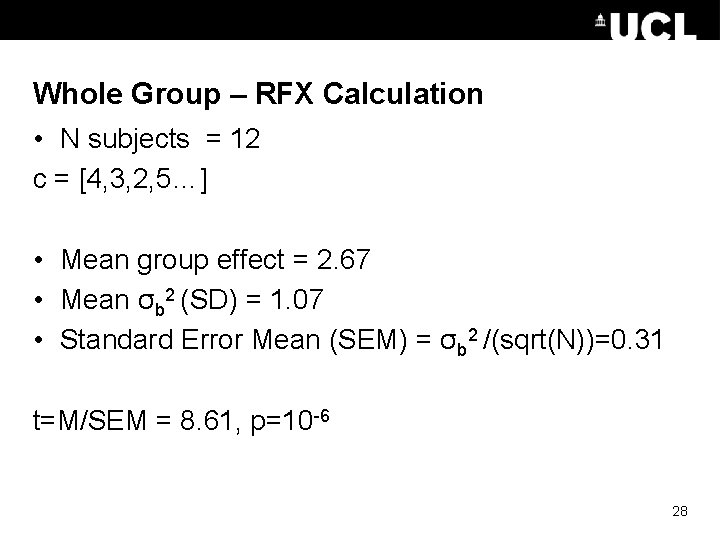
Whole Group – RFX Calculation • N subjects = 12 c = [4, 3, 2, 5…] • Mean group effect = 2. 67 • Mean σb 2 (SD) = 1. 07 • Standard Error Mean (SEM) = σb 2 /(sqrt(N))=0. 31 t=M/SEM = 8. 61, p=10 -6 28

First level Design Matrix Contrast Images One-sample t-test @ second level Subject N … Subject 1 f. MRI data Second level 29 Generalisability, Random Effects & Population Inference. Holmes & Friston, Neuro. Image, 1998.

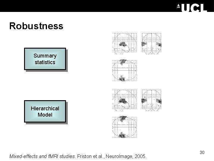
Robustness Summary statistics Hierarchical Model Mixed-effects and f. MRI studies. Friston et al. , Neuro. Image, 2005. 30

Overview of today’s talk 1. 2. 3. 4. 5. 6. Recap of first level analysis What is second level analysis? Fixed vs. random effects How do we analyse random effects? Practical demonstration Questions 31

Buttonpressing 32

33

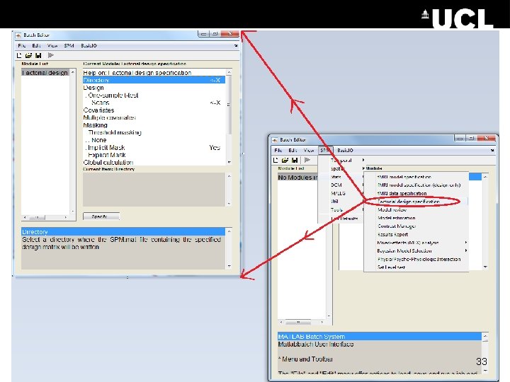
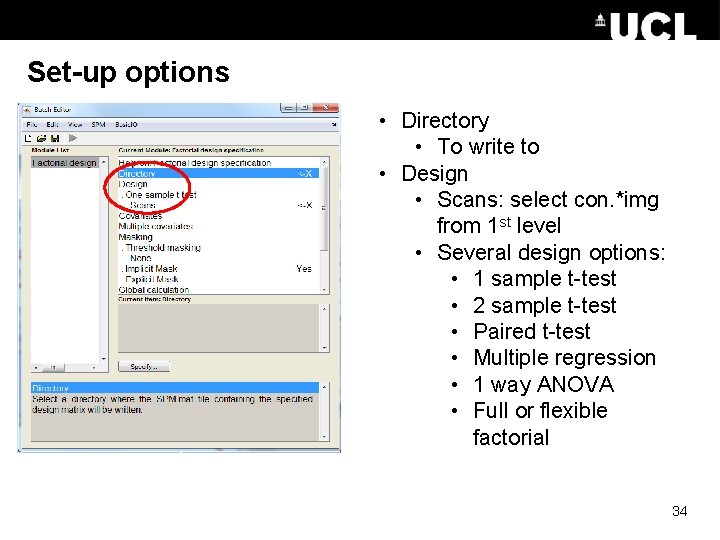
Set-up options • Directory • To write to • Design • Scans: select con. *img from 1 st level • Several design options: • 1 sample t-test • 2 sample t-test • Paired t-test • Multiple regression • 1 way ANOVA • Full or flexible factorial 34

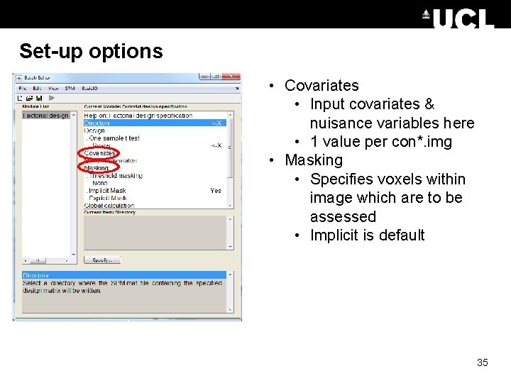
Set-up options • Covariates • Input covariates & nuisance variables here • 1 value per con*. img • Masking • Specifies voxels within image which are to be assessed • Implicit is default 35

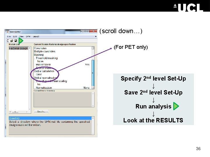
(scroll down…) (For PET only) Specify 2 nd level Set-Up ↓ Save 2 nd level Set-Up ↓ Run analysis ↓ Look at the RESULTS 36

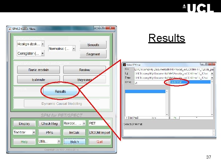
Results 37

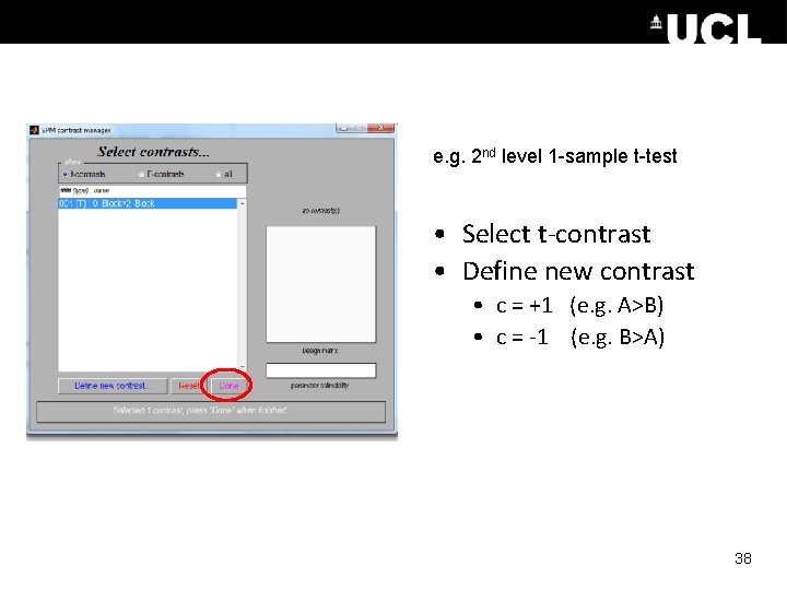
e. g. 2 nd level 1 -sample t-test • Select t-contrast • Define new contrast • c = +1 (e. g. A>B) • c = -1 (e. g. B>A) 38

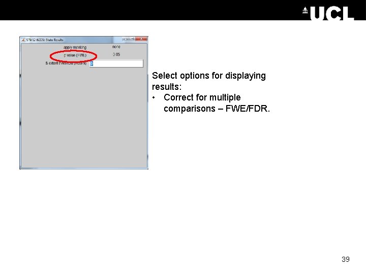
Select options for displaying results: • Correct for multiple comparisons – FWE/FDR. 39

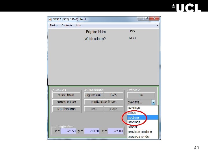
40

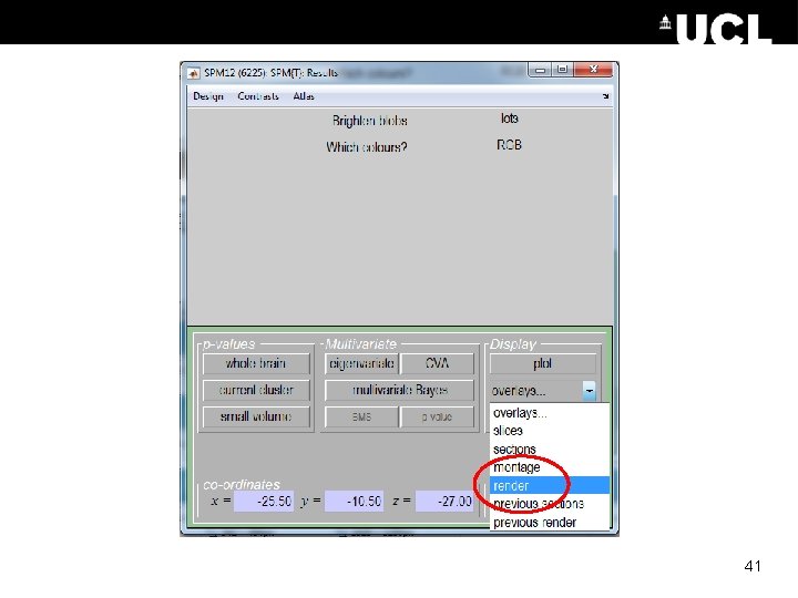
41

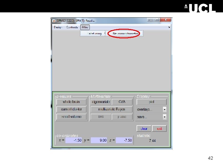
42

Summary • For f. MRI data, usually preferable to use RFX analysis, not FFX • Hierarchical models provide gold standard for RFX , BUT computationally intensive • Summary statistics = robust method for RFX group analysis 43

Overview of today’s talk 1. 2. 3. 4. 5. 6. Recap of first level analysis What is second level analysis? Fixed vs. random effects How do we analyse random effects? Practical demonstration Questions 44

Resources • • Previous Mf. D slides (Bex Bond and Samira Kazan) (Camilla Clark and Cat Slattery) Slides from Guillaume Flandin’s talk in Zurich, Feb 2014 Mumford, J. A. , & Poldrack, R. A. (2007). Modeling group f. MRI data. Social cognitive and affective neuroscience, 2(3), 251 -257. Friston, K. J. , Stephan, K. E. , Lund, T. E. , Morcom, A. , & Kiebel, S. (2005). Mixed-effects and f. MRI studies. Neuroimage, 24(1), 244 -252.