Maximum Likelihood Estimation Expectation Maximization Lectures 3 Oct

Maximum Likelihood Estimation & Expectation Maximization Lectures 3 – Oct 5, 2011 CSE 527 Computational Biology, Fall 2011 Instructor: Su-In Lee TA: Christopher Miles Monday & Wednesday 12: 00 -1: 20 Johnson Hall (JHN) 022 1

Outline n Probabilistic models in biology n Model selection problem n Mathematical foundations n Bayesian networks n Learning from data n n n Maximum likelihood estimation Maximum a posteriori (MAP) Expectation and maximization 2

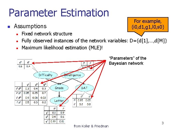
Parameter Estimation n Assumptions n n n For example, {i 0, d 1, g 1, l 0, s 0} Fixed network structure Fully observed instances of the network variables: D={d[1], …, d[M]} Maximum likelihood estimation (MLE)! “Parameters” of the Bayesian network from Koller & Friedman 3

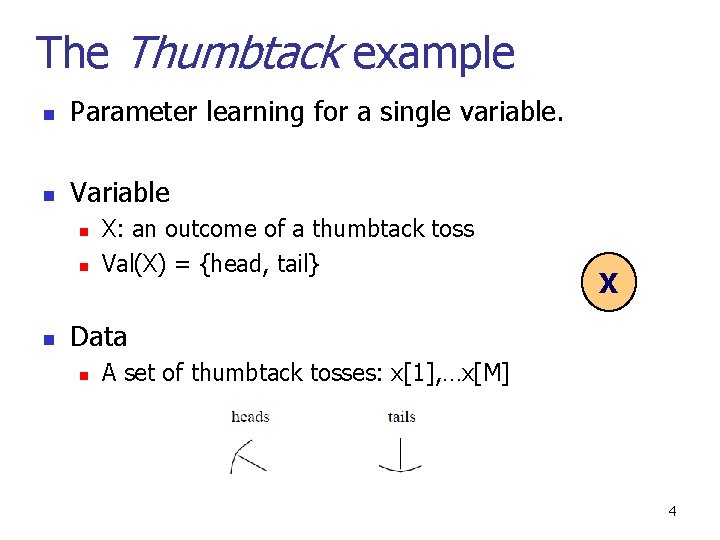
The Thumbtack example n Parameter learning for a single variable. n Variable n n n X: an outcome of a thumbtack toss Val(X) = {head, tail} X Data n A set of thumbtack tosses: x[1], …x[M] 4

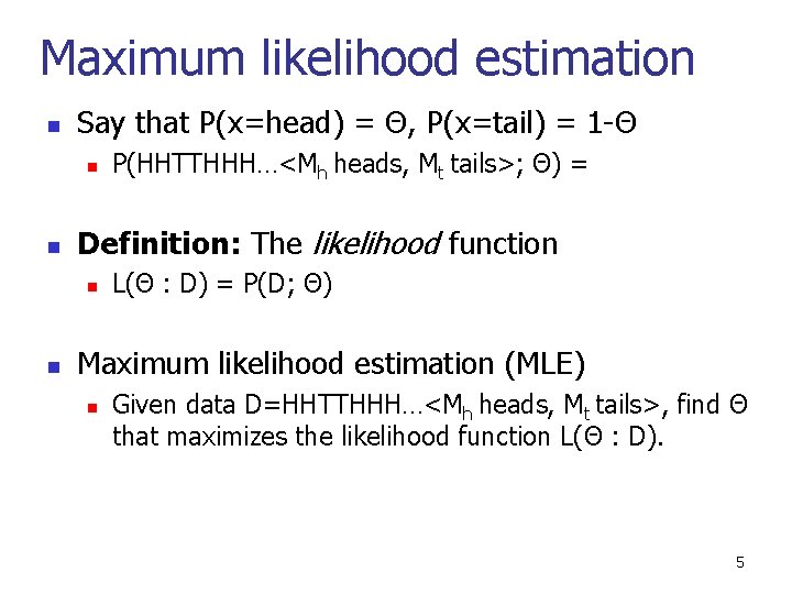
Maximum likelihood estimation n Say that P(x=head) = Θ, P(x=tail) = 1 -Θ n n Definition: The likelihood function n n P(HHTTHHH…<Mh heads, Mt tails>; Θ) = L(Θ : D) = P(D; Θ) Maximum likelihood estimation (MLE) n Given data D=HHTTHHH…<Mh heads, Mt tails>, find Θ that maximizes the likelihood function L(Θ : D). 5

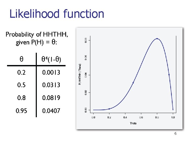
Likelihood function 6

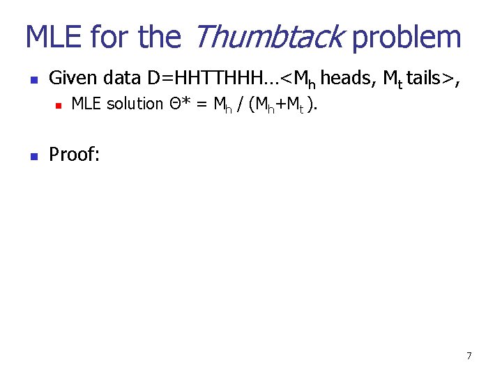
MLE for the Thumbtack problem n Given data D=HHTTHHH…<Mh heads, Mt tails>, n n MLE solution Θ* = Mh / (Mh+Mt ). Proof: 7

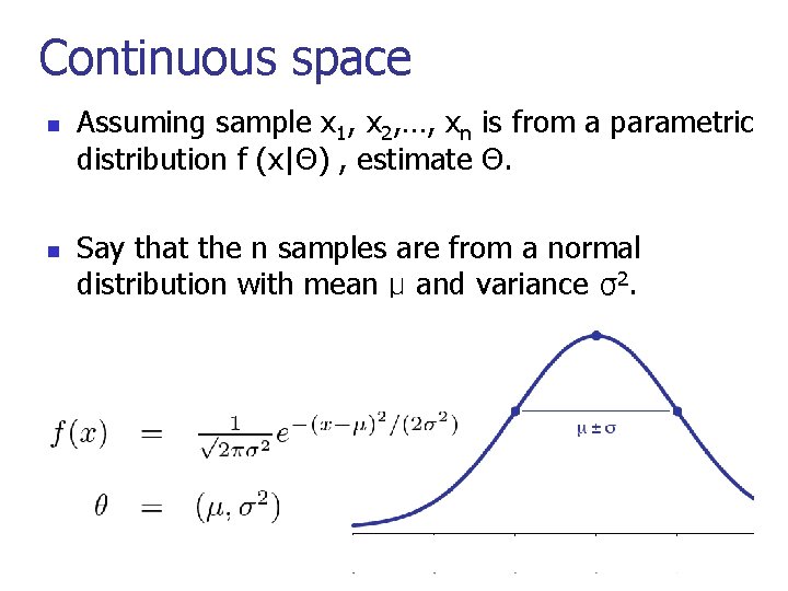
Continuous space n n Assuming sample x 1, x 2, …, xn is from a parametric distribution f (x|Θ) , estimate Θ. Say that the n samples are from a normal distribution with mean μ and variance σ2. 8

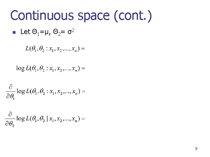
Continuous space (cont. ) n Let Θ 1=μ, Θ 2= σ2 9

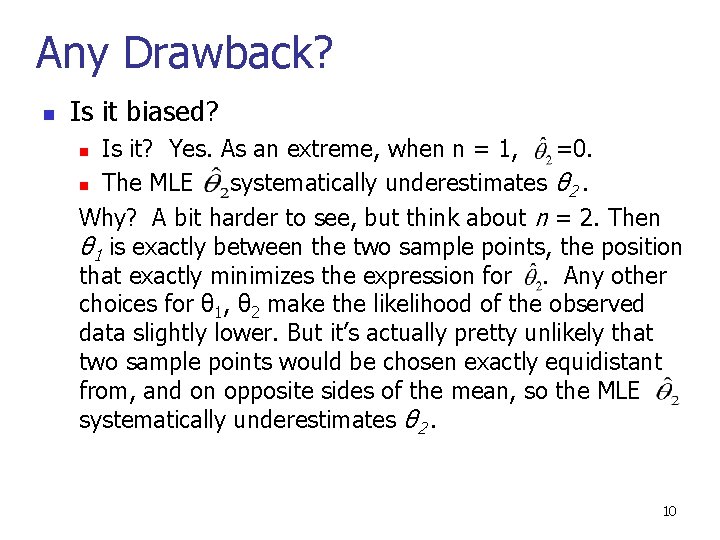
Any Drawback? n Is it biased? Is it? Yes. As an extreme, when n = 1, =0. n The MLE systematically underestimates θ 2. Why? A bit harder to see, but think about n = 2. Then θ 1 is exactly between the two sample points, the position that exactly minimizes the expression for. Any other choices for θ 1, θ 2 make the likelihood of the observed data slightly lower. But it’s actually pretty unlikely that two sample points would be chosen exactly equidistant from, and on opposite sides of the mean, so the MLE systematically underestimates θ 2. n 10

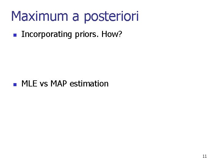
Maximum a posteriori n Incorporating priors. How? n MLE vs MAP estimation 11

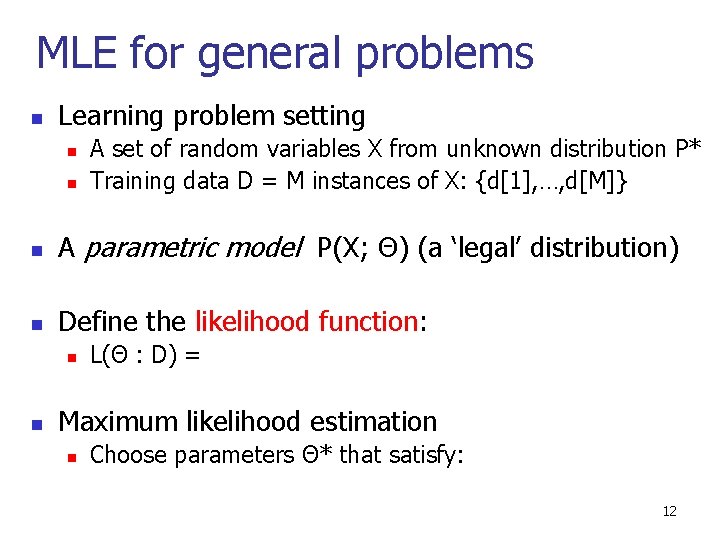
MLE for general problems n Learning problem setting n n A set of random variables X from unknown distribution P* Training data D = M instances of X: {d[1], …, d[M]} n A parametric model P(X; Θ) (a ‘legal’ distribution) n Define the likelihood function: n n L(Θ : D) = Maximum likelihood estimation n Choose parameters Θ* that satisfy: 12

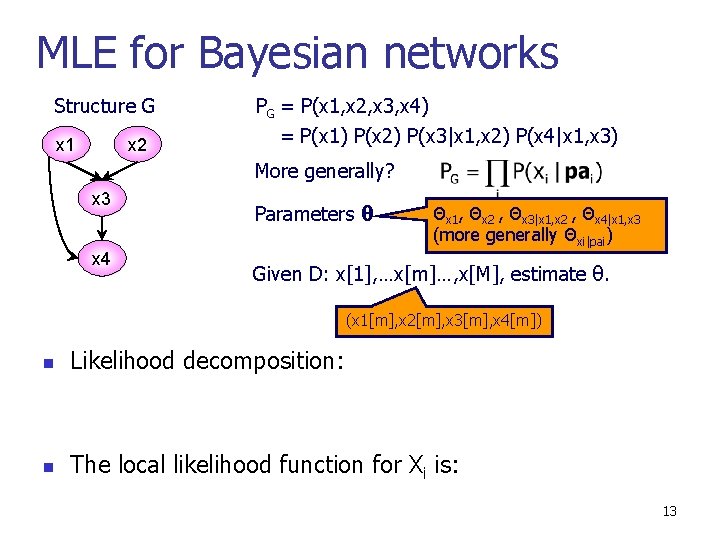
MLE for Bayesian networks Structure G x 1 x 2 PG = P(x 1, x 2, x 3, x 4) = P(x 1) P(x 2) P(x 3|x 1, x 2) P(x 4|x 1, x 3) More generally? x 3 x 4 Parameters θ Θx 1, Θx 2 , Θx 3|x 1, x 2 , Θx 4|x 1, x 3 (more generally Θxi|pai) Given D: x[1], …x[m]…, x[M], estimate θ. (x 1[m], x 2[m], x 3[m], x 4[m]) n Likelihood decomposition: n The local likelihood function for Xi is: 13

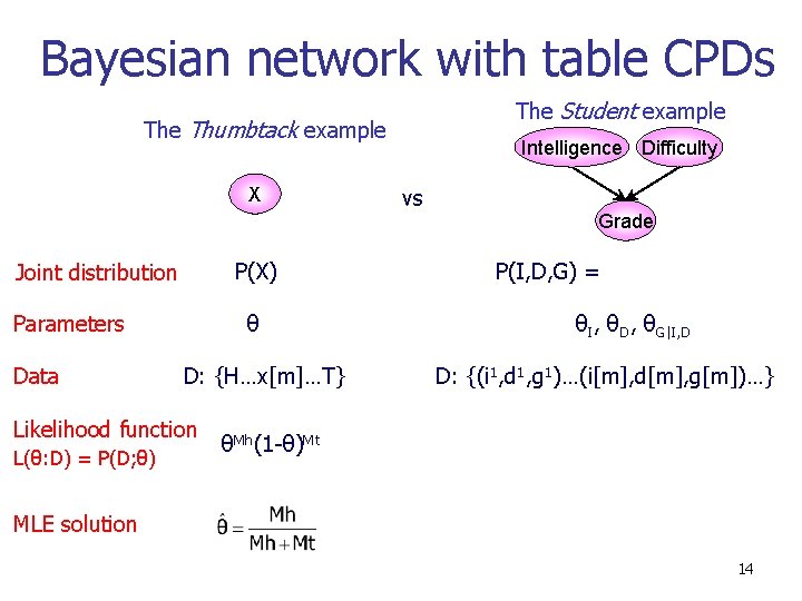
Bayesian network with table CPDs The Student example Thumbtack example X P(X) Joint distribution Parameters Data θ D: {H…x[m]…T} Likelihood function L(θ: D) = P(D; θ) Intelligence Difficulty vs Grade P(I, D, G) = θI, θD, θG|I, D D: {(i 1, d 1, g 1)…(i[m], d[m], g[m])…} θMh(1 -θ)Mt MLE solution 14

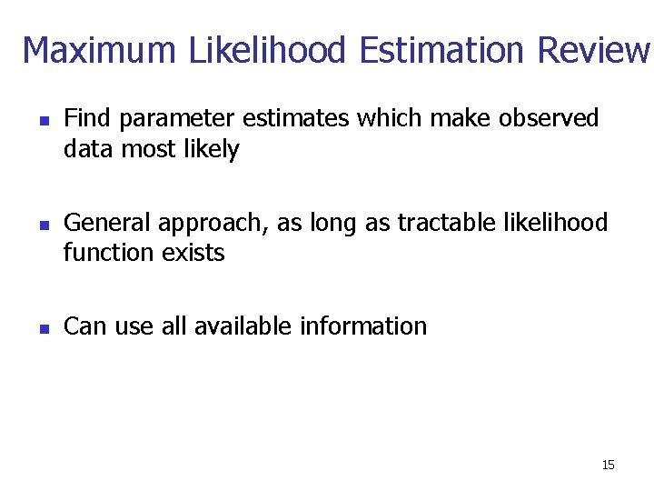
Maximum Likelihood Estimation Review n n n Find parameter estimates which make observed data most likely General approach, as long as tractable likelihood function exists Can use all available information 15

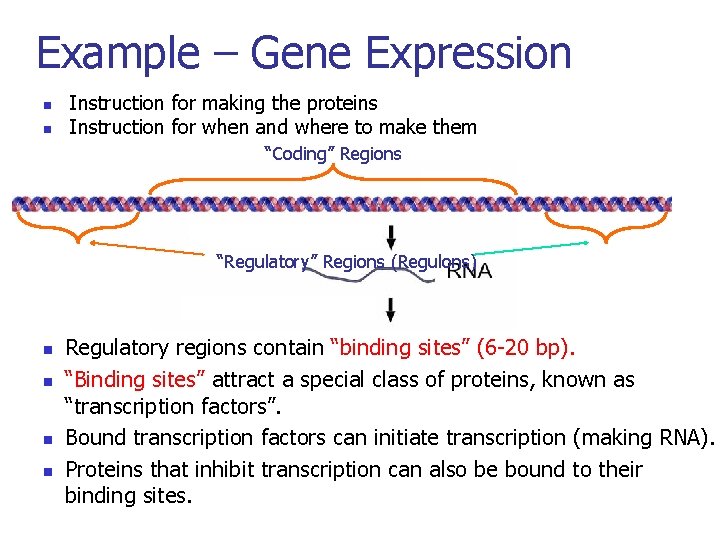
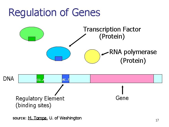
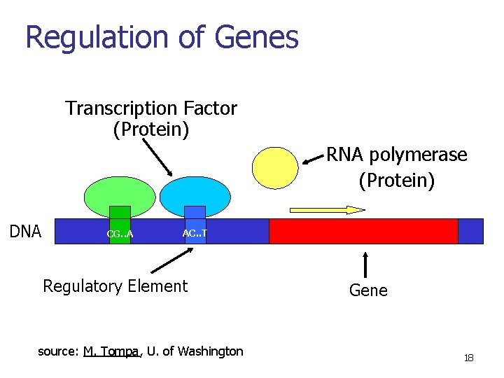
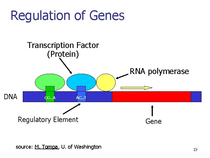
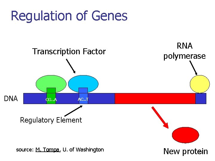
Example – Gene Expression n n Instruction for making the proteins Instruction for when and where to make them “Coding” Regions “Regulatory” Regions (Regulons) n n n n Regulatory regions contain “binding sites” (6 -20 bp). “Binding sites” attract a special class of proteins, known as “transcription factors”. What turns genes on (producing a protein) and off? Bound factors can initiate transcription (making RNA). When istranscription a gene turned on or off? Proteins inhibit canon? also be bound to their Where (inthat which cells)transcription is a gene turned binding sites. How many copies of the gene product are produced? 16

Regulation of Genes Transcription Factor (Protein) RNA polymerase (Protein) DNA CG. . A AC. . T Regulatory Element (binding sites) source: M. Tompa, U. of Washington Gene 17

Regulation of Genes Transcription Factor (Protein) RNA polymerase (Protein) DNA CG. . A AC. . T Regulatory Element source: M. Tompa, U. of Washington Gene 18

Regulation of Genes Transcription Factor (Protein) RNA polymerase DNA CG. . A AC. . T Regulatory Element source: M. Tompa, U. of Washington Gene 19

Regulation of Genes Transcription Factor DNA CG. . A RNA polymerase AC. . T Regulatory Element source: M. Tompa, U. of Washington 20 New protein

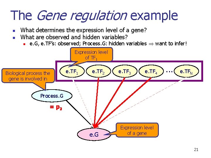
The Gene regulation example n n What determines the expression level of a gene? What are observed and hidden variables? n e. G, e. TF’s: observed; Process. G: hidden variables want to infer! Expression level of TF 1 Biological process the gene is involved in e. TF 1 e. TF 2 e. TF 3 e. TF 4 . . . e. TFN Process. G = p 321 e. G Expression level of a gene 21

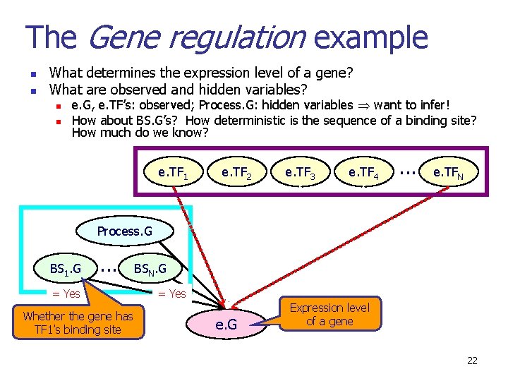
The Gene regulation example n n What determines the expression level of a gene? What are observed and hidden variables? n n e. G, e. TF’s: observed; Process. G: hidden variables want to infer! How about BS. G’s? How deterministic is the sequence of a binding site? How much do we know? e. TF 1 e. TF 2 e. TF 3 e. TF 4 . . . e. TFN Process. G BS 1. G . . . = Yes Whether the gene has TF 1’s binding site BSN. G = Yes e. G Expression level of a gene 22

Not all data are perfect n n Most MLE problems are simple to solve with complete data. Available data are “incomplete” in some way. 23

Outline n Learning from data n n n Maximum likelihood estimation (MLE) Maximum a posteriori (MAP) Expectation-maximization (EM) algorithm 24

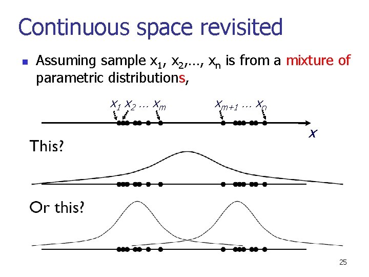
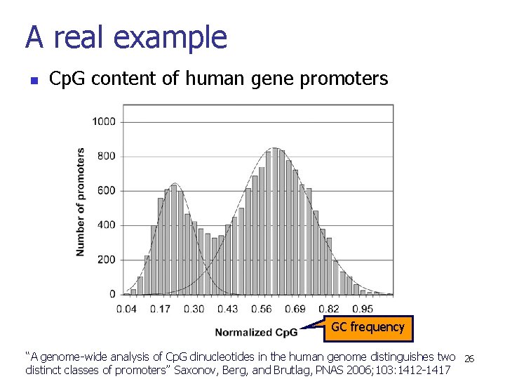
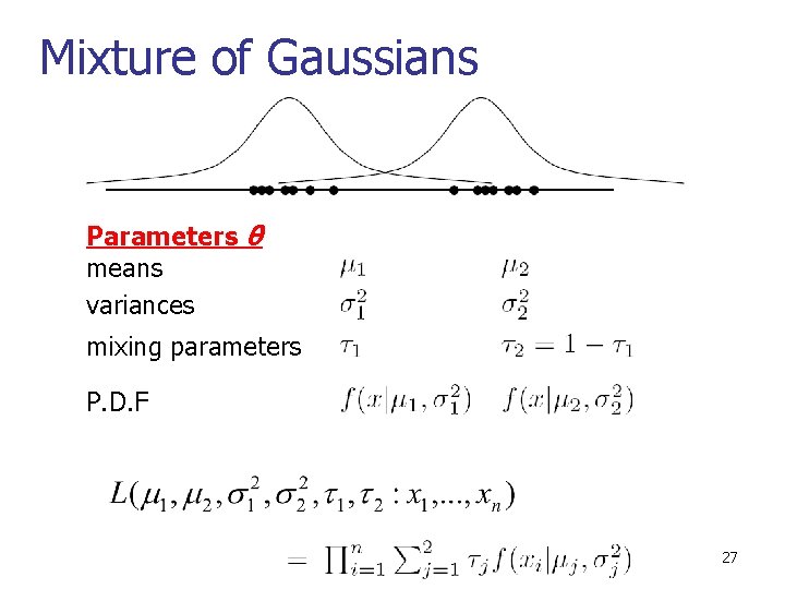
Continuous space revisited n Assuming sample x 1, x 2, …, xn is from a mixture of parametric distributions, x 1 x 2 … x m xm+1 … xn x 25

A real example n Cp. G content of human gene promoters GC frequency “A genome-wide analysis of Cp. G dinucleotides in the human genome distinguishes two 26 distinct classes of promoters” Saxonov, Berg, and Brutlag, PNAS 2006; 103: 1412 -1417

Mixture of Gaussians Parameters θ means variances mixing parameters P. D. F 27

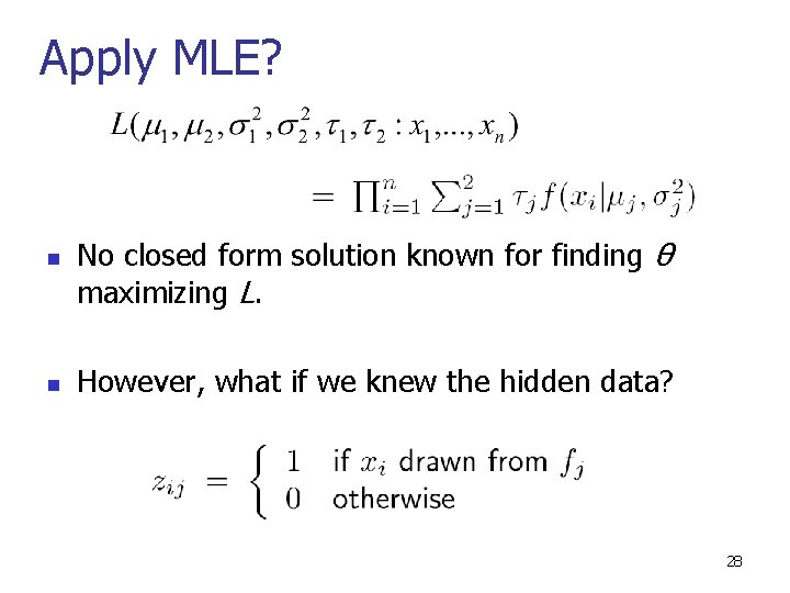
Apply MLE? n n No closed form solution known for finding θ maximizing L. However, what if we knew the hidden data? 28

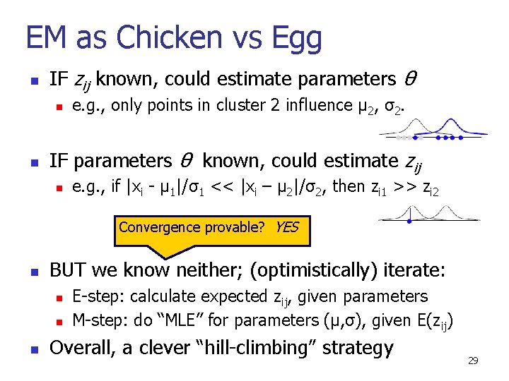
EM as Chicken vs Egg n IF zij known, could estimate parameters θ n n e. g. , only points in cluster 2 influence μ 2, σ2. IF parameters θ known, could estimate zij n e. g. , if |xi - μ 1|/σ1 << |xi – μ 2|/σ2, then zi 1 >> zi 2 Convergence provable? YES n BUT we know neither; (optimistically) iterate: n n n E-step: calculate expected zij, given parameters M-step: do “MLE” for parameters (μ, σ), given E(zij) Overall, a clever “hill-climbing” strategy 29

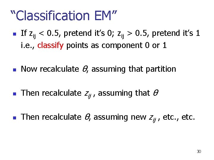
“Classification EM” n If zij < 0. 5, pretend it’s 0; zij > 0. 5, pretend it’s 1 i. e. , classify points as component 0 or 1 n Now recalculate θ, assuming that partition n Then recalculate zij , assuming that θ n Then recalculate θ, assuming new zij , etc. 30

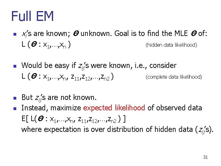
Full EM n n xi’s are known; Θ unknown. Goal is to find the MLE Θ of: L (Θ : x 1, …, xn ) (hidden data likelihood) Would be easy if zij’s were known, i. e. , consider L (Θ : x 1, …, xn, z 11, z 12, …, zn 2 ) (complete data likelihood) But zij’s are not known. Instead, maximize expected likelihood of observed data E[ L(Θ : x 1, …, xn, z 11, z 12, …, zn 2 ) ] where expectation is over distribution of hidden data (zij’s). 31

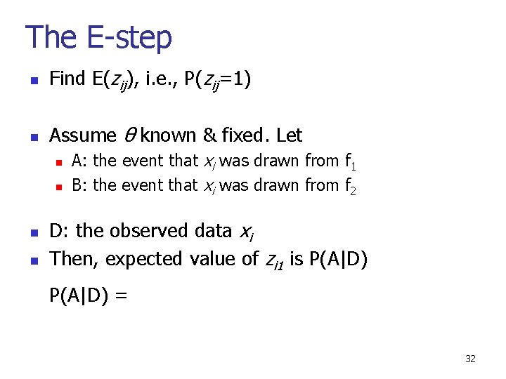
The E-step n Find E(zij), i. e. , P(zij=1) n Assume θ known & fixed. Let n n A: the event that xi was drawn from f 1 B: the event that xi was drawn from f 2 D: the observed data xi Then, expected value of zi 1 is P(A|D) = 32

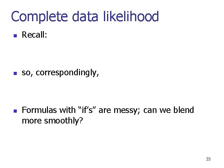
Complete data likelihood n Recall: n so, correspondingly, n Formulas with “if’s” are messy; can we blend more smoothly? 33

M-step n Find θ maximizing E[ log(Likelihood) ] 34

EM summary n Fundamentally an MLE problem n Useful if analysis is more tractable when 0/1 n Hidden data z known n Iterate: E-step: estimate E(z) for each z, given θ M-step: estimate θ maximizing E(log likelihood) given E(z) where “E(log. L)” is wrt random z ~ E(z) = p(z=1) 35

EM Issues n n EM is guaranteed to increase likelihood with every E-M iteration, hence will converge. But may converge to local, not global, max. Issue is intrinsic (probably), since EM is often applied to NP-hard problems (including clustering, above, and motif-discovery, soon) Nevertheless, widely used, often effective 36

Acknowledgement n Profs Daphne Koller & Nir Friedman, “Probabilistic Graphical Models” n Prof Larry Ruzo, CSE 527, Autumn 2009 n Prof Andrew Ng, ML lecture note 37