Lecture 4 The Simplex Method Last Lectures Summary

Lecture 4 The Simplex Method

Last Lecture’s Summary • Covered Sec. 11. 1: Simplex Preliminaries • Requirements of Simplex Method • Requirement – I for different types of constraints • Feasible Solution, Basic Solution, and Basic Feasible Solution

Today • We start Sec 11. 2: The Simplex Method • Solution (of constraint equations) by Enumeration • Then, incorporating the objective function • Rules 1, 2, and 3 in Maximization problem • Examples

THE SIMPLEX METHOD Before we begin our discussions of the simplex method, let’s provide a generalized statement of an LP model. Given the definitions xj = jth decision variable cj = coefficient on jth decision variable in the objective function. aij = coefficient in the ith constraint for the jth variable. bi = right-hand-side constant for the ith constraint

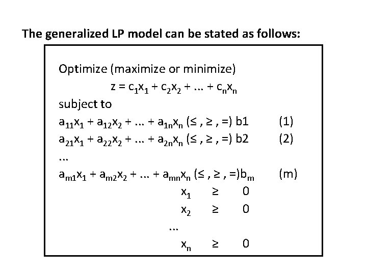
The generalized LP model can be stated as follows: Optimize (maximize or minimize) z = c 1 x 1 + c 2 x 2 +. . . + cnxn subject to a 11 x 1 + a 12 x 2 +. . . + a 1 nxn (≤ , ≥ , =) b 1 a 21 x 1 + a 22 x 2 +. . . + a 2 nxn (≤ , ≥ , =) b 2. . . am 1 x 1 + am 2 x 2 +. . . + amnxn (≤ , ≥ , =)bm x 1 ≥ 0 x 2 ≥ 0. . . xn ≥ 0 (1) (2) (m)

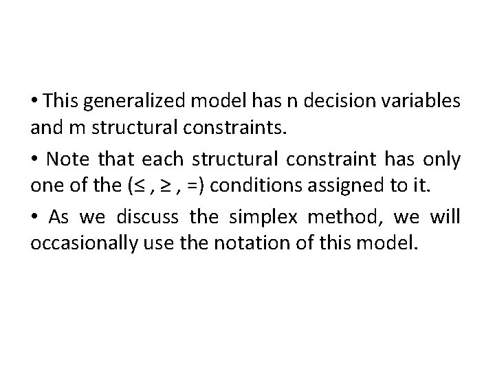
• This generalized model has n decision variables and m structural constraints. • Note that each structural constraint has only one of the (≤ , ≥ , =) conditions assigned to it. • As we discuss the simplex method, we will occasionally use the notation of this model.

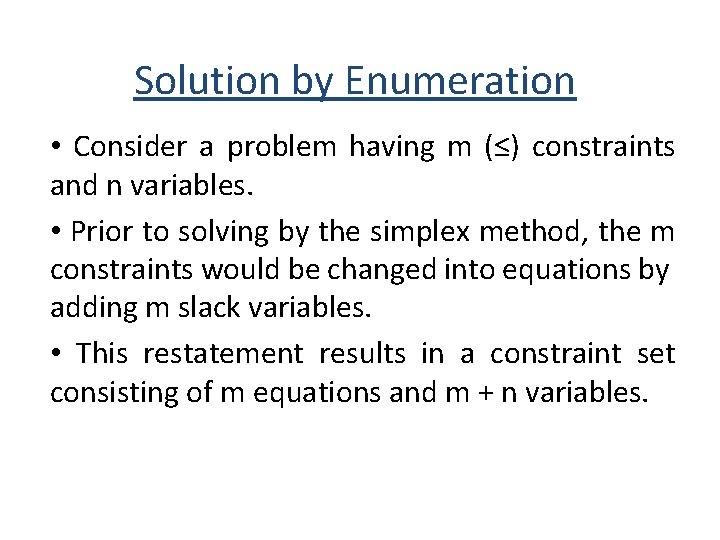
Solution by Enumeration • Consider a problem having m (≤) constraints and n variables. • Prior to solving by the simplex method, the m constraints would be changed into equations by adding m slack variables. • This restatement results in a constraint set consisting of m equations and m + n variables.

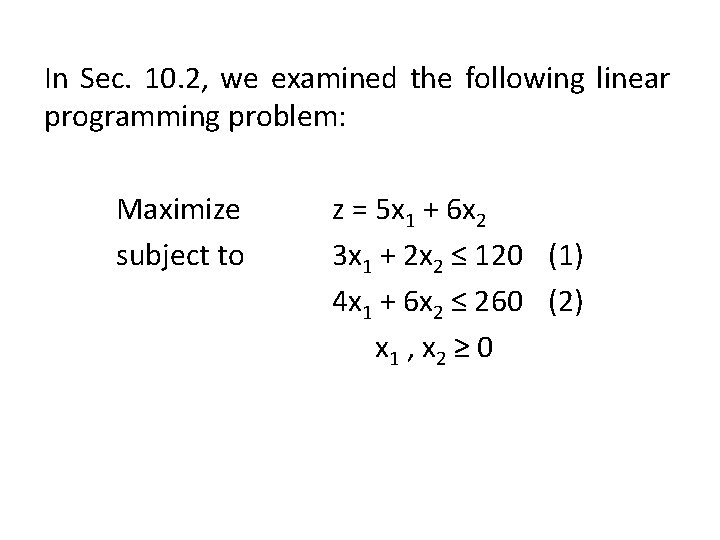
In Sec. 10. 2, we examined the following linear programming problem: Maximize subject to z = 5 x 1 + 6 x 2 3 x 1 + 2 x 2 ≤ 120 (1) 4 x 1 + 6 x 2 ≤ 260 (2) x 1 , x 2 ≥ 0

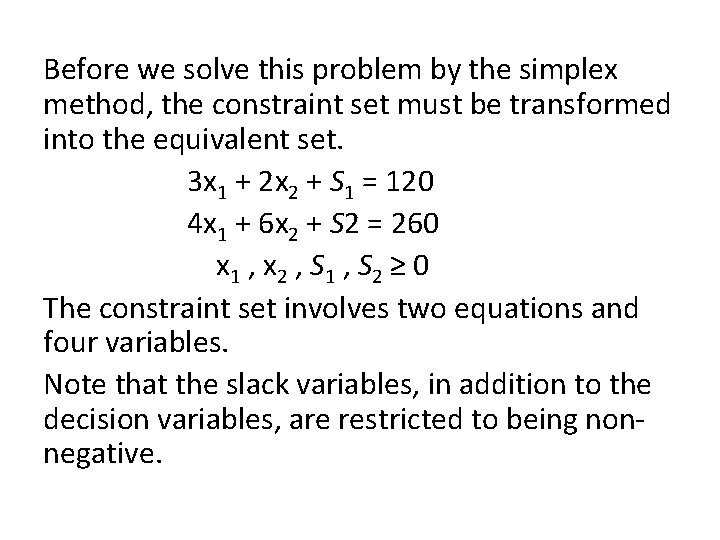
Before we solve this problem by the simplex method, the constraint set must be transformed into the equivalent set. 3 x 1 + 2 x 2 + S 1 = 120 4 x 1 + 6 x 2 + S 2 = 260 x 1 , x 2 , S 1 , S 2 ≥ 0 The constraint set involves two equations and four variables. Note that the slack variables, in addition to the decision variables, are restricted to being nonnegative.

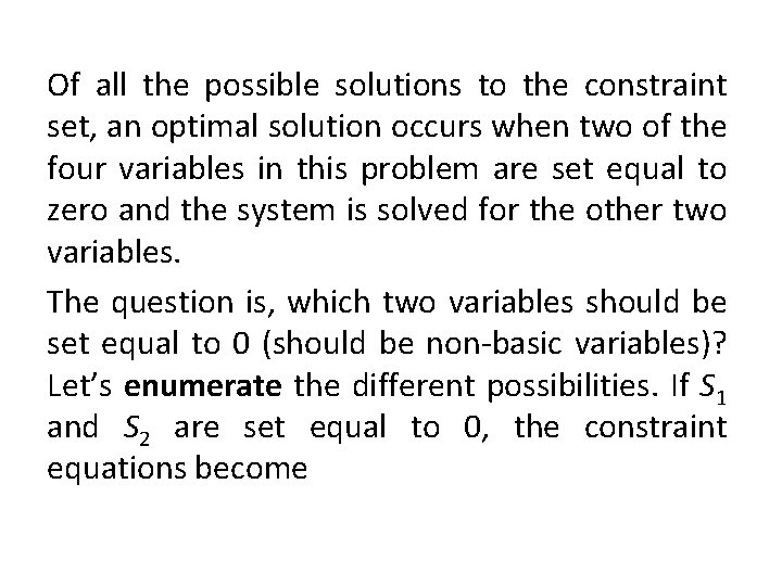
Of all the possible solutions to the constraint set, an optimal solution occurs when two of the four variables in this problem are set equal to zero and the system is solved for the other two variables. The question is, which two variables should be set equal to 0 (should be non-basic variables)? Let’s enumerate the different possibilities. If S 1 and S 2 are set equal to 0, the constraint equations become

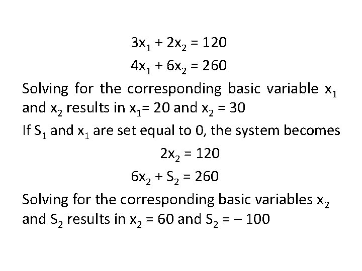
3 x 1 + 2 x 2 = 120 4 x 1 + 6 x 2 = 260 Solving for the corresponding basic variable x 1 and x 2 results in x 1= 20 and x 2 = 30 If S 1 and x 1 are set equal to 0, the system becomes 2 x 2 = 120 6 x 2 + S 2 = 260 Solving for the corresponding basic variables x 2 and S 2 results in x 2 = 60 and S 2 = – 100

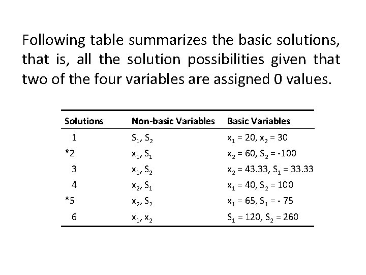
Following table summarizes the basic solutions, that is, all the solution possibilities given that two of the four variables are assigned 0 values. Solutions Non-basic Variables Basic Variables 1 S 1 , S 2 x 1 = 20, x 2 = 30 *2 x 1 , S 1 x 2 = 60, S 2 = -100 3 x 1 , S 2 x 2 = 43. 33, S 1 = 33. 33 4 x 2 , S 1 x 1 = 40, S 2 = 100 *5 x 2 , S 2 x 1 = 65, S 1 = - 75 6 x 1 , x 2 S 1 = 120, S 2 = 260

Notice that solutions 2 and 5 are not feasible. They each contain a variable which has a negative value, violating the non-negativity restriction. However, solutions 1, 3, 4 and 6 are basic feasible solutions to the linear programming problem and are candidates for the optimal solution.

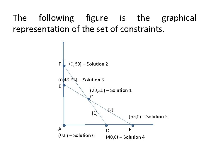
The following figure is the graphical representation of the set of constraints. F (0, 60) – Solution 2 (0, 43. 33) – Solution 3 B (20, 30) – Solution 1 C (1) A (0, 6) – Solution 6 (2) (65, 0) – Solution 5 E D (40, 0) – Solution 4

In this figure the points of intersection (A, B, C, D, E, F) between the structural constraint lines and the non-negativity constraints (x 1 and x 2 axes) represent the set of basic solutions. Solutions 1, 3, 4 and 6 in the table above are the basic feasible solutions and correspond to the four corner points on the region of feasible solutions in the figure.

Specifically, solution 1 corresponds to corner point C, solution 3 corresponds to corner point B, solution 4 corresponds to corner point D, and solution 6 corresponds to corner point A. Solution 2 and 5, which are not feasible, correspond to points E and F shown in the figure.

The important thing to note is that by setting all combinations of two different variables equal to 0 and solving for the remaining variables, a set of potential solutions (basic solutions) was identified for the LP problem. A subset of these solutions was automatically disqualified because it contained infeasible solutions (2 and 5).

However, the remaining basic feasible solutions corresponded to the corner points on the region of feasible solutions. Since we know that an optimal solution will occur at ‘at least’ one of these corner points, further examination of these will reveal an optimal solution.

For a maximization problem having m (≤) constraints and n decision variables, the addition of m slack variables results in m constraint equations containing m + n variables. An optimal solution to this problem can be found by setting n of the variables equal to 0 and solving for the remaining m variables.

In the process of selecting different combinations of n variables to be set equal to 0, the simplex • will never select a combination which will result in an infeasible solution and • will ensure that each new combination selected will result in a solution which has an objective function value at least as good as the current solution.

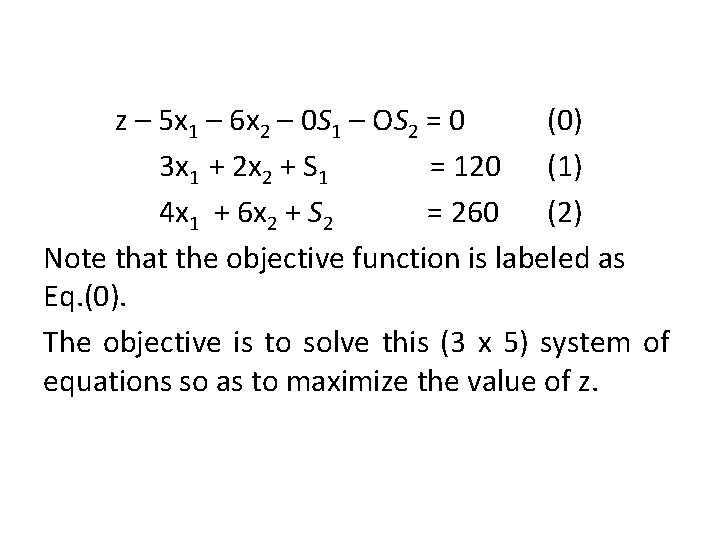
Incorporating the Objective Function In solving by the simplex method, the objective function and constraints are combined to form a system of equations. The objective function is one of the equations, and z becomes an additional variable in the system. In rearranging the variables in the objective function so that they are all on the left side of the equation, the problem is represented by the system of equations.

z – 5 x 1 – 6 x 2 – 0 S 1 – OS 2 = 0 (0) 3 x 1 + 2 x 2 + S 1 = 120 (1) 4 x 1 + 6 x 2 + S 2 = 260 (2) Note that the objective function is labeled as Eq. (0). The objective is to solve this (3 x 5) system of equations so as to maximize the value of z.

Since we are particularly concerned about the value of z and will want to know its value for any solution, z will always be a basic variable. The standard practice, however, is not to refer to z as a basic variable. The terms basic variable and non-basic variable are usually reserved for other variables in the problem.

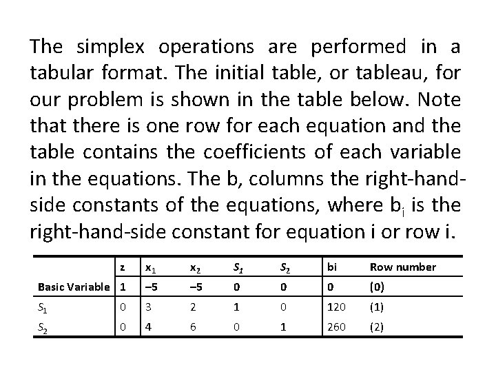
The simplex operations are performed in a tabular format. The initial table, or tableau, for our problem is shown in the table below. Note that there is one row for each equation and the table contains the coefficients of each variable in the equations. The b, columns the right-handside constants of the equations, where bi is the right-hand-side constant for equation i or row i. z x 1 x 2 S 1 S 2 bi Row number Basic Variable 1 – 5 0 0 0 (0) S 1 0 3 2 1 0 120 (1) S 2 0 4 6 0 1 260 (2)

RULE: 1 OPTIMALITY CHECK IN MAXIMIZATION PROBLEM In a maximization problem, the optimal solution has been found if all row (0) coefficients for the variables are greater than or equal to 0. If any row (0) coefficients are negative for non-basic variable, a better solution can be found by assigning a positive quantity to these variables.

RULE: 2 NEW BASIC VARIABLE IN MAXIMIZATION PROBLEM In a maximization problem the non-basic variable which will replace a basic variable is the one having the most negative row (0) coefficient. “Ties” may be broken arbitrarily.

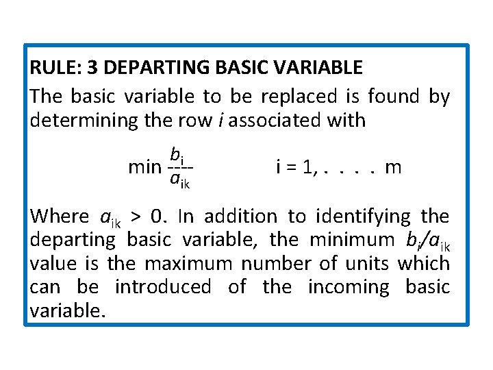
RULE: 3 DEPARTING BASIC VARIABLE The basic variable to be replaced is found by determining the row i associated with bi min ---aik i = 1, . . m Where aik > 0. In addition to identifying the departing basic variable, the minimum bi/aik value is the maximum number of units which can be introduced of the incoming basic variable.

SUMMARY OF SIMPLEX PROCEDURE Let’s generalize the simplex procedure for maximization problems having all (≤) constraints. First, add slack variables to each constraint and the objective function and place the variable coefficients and right-hand-side constants in a simplex tableau:

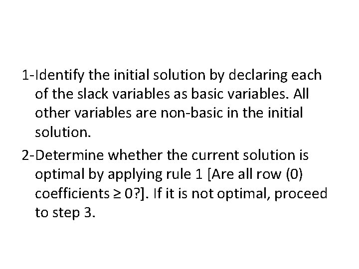
1 -Identify the initial solution by declaring each of the slack variables as basic variables. All other variables are non-basic in the initial solution. 2 -Determine whether the current solution is optimal by applying rule 1 [Are all row (0) coefficients ≥ 0? ]. If it is not optimal, proceed to step 3.

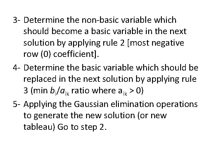
3 - Determine the non-basic variable which should become a basic variable in the next solution by applying rule 2 [most negative row (0) coefficient]. 4 - Determine the basic variable which should be replaced in the next solution by applying rule 3 (min bi/aik ratio where aik > 0) 5 - Applying the Gaussian elimination operations to generate the new solution (or new tableau) Go to step 2.

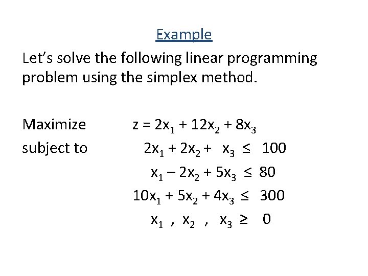
Example Let’s solve the following linear programming problem using the simplex method. Maximize subject to z = 2 x 1 + 12 x 2 + 8 x 3 2 x 1 + 2 x 2 + x 3 ≤ 100 x 1 – 2 x 2 + 5 x 3 ≤ 80 10 x 1 + 5 x 2 + 4 x 3 ≤ 300 x 1 , x 2 , x 3 ≥ 0

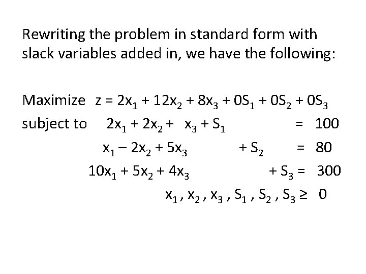
Rewriting the problem in standard form with slack variables added in, we have the following: Maximize z = 2 x 1 + 12 x 2 + 8 x 3 + 0 S 1 + 0 S 2 + 0 S 3 subject to 2 x 1 + 2 x 2 + x 3 + S 1 = 100 x 1 – 2 x 2 + 5 x 3 + S 2 = 80 10 x 1 + 5 x 2 + 4 x 3 + S 3 = 300 x 1 , x 2 , x 3 , S 1 , S 2 , S 3 ≥ 0

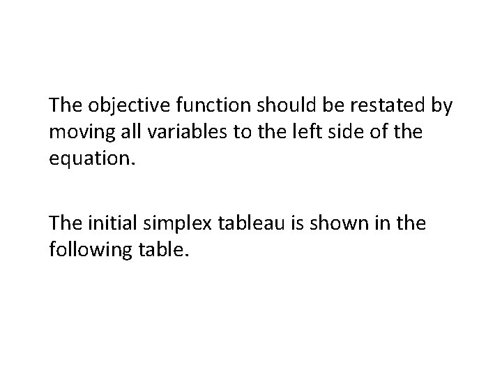
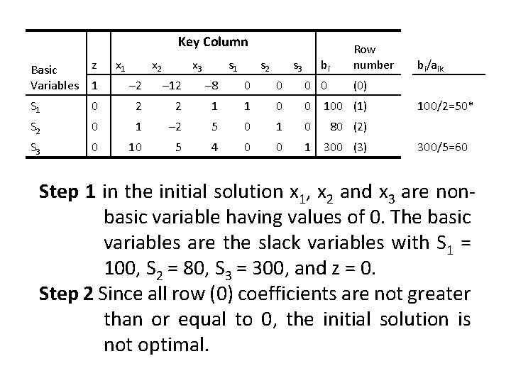
The objective function should be restated by moving all variables to the left side of the equation. The initial simplex tableau is shown in the following table.

Key Column x 1 x 2 x 3 s 1 s 2 s 3 bi Row number Basic Variables z 1 – 2 – 12 – 8 0 0 S 1 0 2 2 1 1 0 0 100 (1) S 2 0 1 – 2 5 0 1 0 80 (2) S 3 0 10 5 4 0 0 1 300 (3) bi/aik (0) 100/2=50* 300/5=60 Step 1 in the initial solution x 1, x 2 and x 3 are nonbasic variable having values of 0. The basic variables are the slack variables with S 1 = 100, S 2 = 80, S 3 = 300, and z = 0. Step 2 Since all row (0) coefficients are not greater than or equal to 0, the initial solution is not optimal.

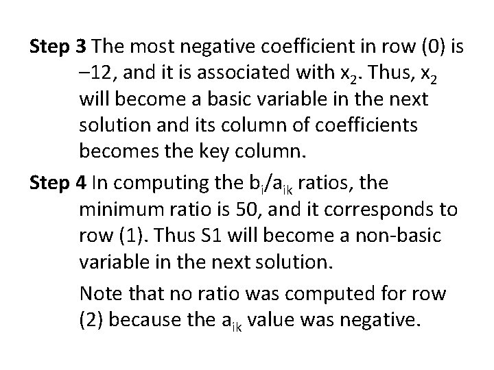
Step 3 The most negative coefficient in row (0) is – 12, and it is associated with x 2. Thus, x 2 will become a basic variable in the next solution and its column of coefficients becomes the key column. Step 4 In computing the bi/aik ratios, the minimum ratio is 50, and it corresponds to row (1). Thus S 1 will become a non-basic variable in the next solution. Note that no ratio was computed for row (2) because the aik value was negative.

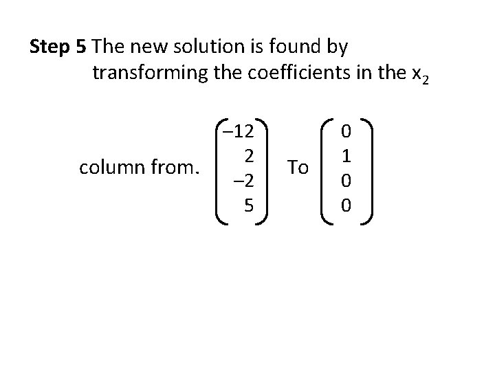
Step 5 The new solution is found by transforming the coefficients in the x 2 column from. – 12 2 – 2 5 To 0 1 0 0

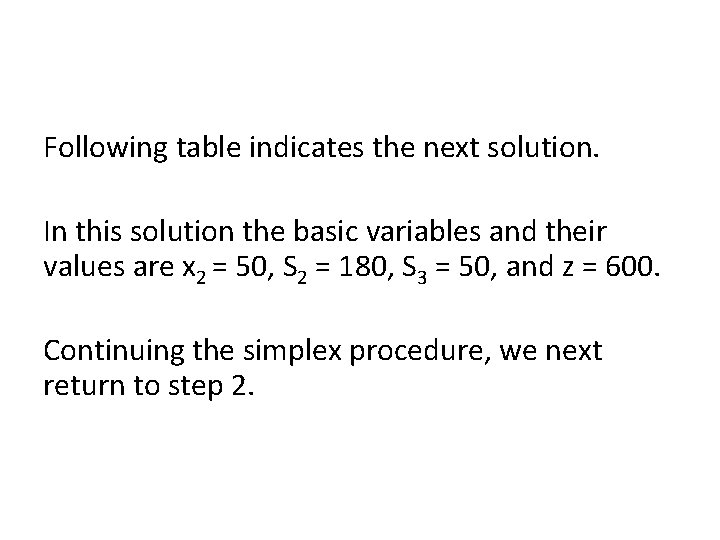
Following table indicates the next solution. In this solution the basic variables and their values are x 2 = 50, S 2 = 180, S 3 = 50, and z = 600. Continuing the simplex procedure, we next return to step 2.

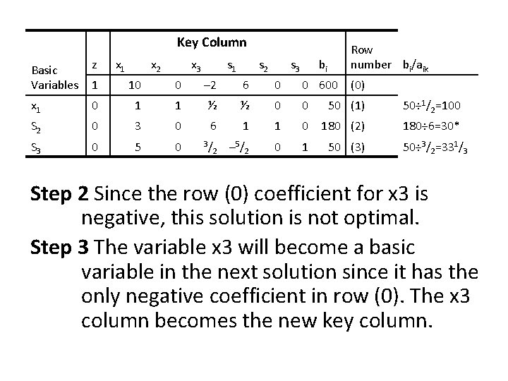
Key Column x 1 x 2 x 3 s 1 Basic Variables z 1 10 0 – 2 6 0 0 600 (0) x 1 0 1 1 ½ ½ 0 0 50 (1) 50÷ 1/2=100 S 2 0 3 0 6 1 1 0 180 (2) 180÷ 6=30* S 3 0 5 0 – 5/2 0 1 50÷ 3/2=331/3 3/ 2 s 3 bi Row number bi/aik 50 (3) Step 2 Since the row (0) coefficient for x 3 is negative, this solution is not optimal. Step 3 The variable x 3 will become a basic variable in the next solution since it has the only negative coefficient in row (0). The x 3 column becomes the new key column.

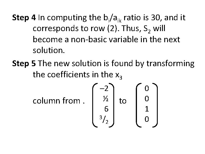
Step 4 In computing the bi/aik ratio is 30, and it corresponds to row (2). Thus, S 2 will become a non-basic variable in the next solution. Step 5 The new solution is found by transforming the coefficients in the x 3 column from. – 2 ½ 6 3/ 2 to 0 0 1 0

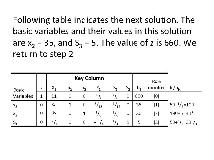
Following table indicates the next solution. The basic variables and their values in this solution are x 2 = 35, and S 3 = 5. The value of z is 660. We return to step 2 Key Column Row number bi/aik Basic Variables z X 1 x 2 x 3 S 1 S 2 S 3 bi 1 11 0 0 38/ 6 2/ 0 660 (0) x 2 0 ¾ 1 0 5/ 12 – 1/12 0 35 (1) 50÷ 1/2=100 x 3 0 ½ 0 1 1/ 1/ 6 0 30 (2) 180÷ 6=30* S 3 0 17/ 0 0 – 11/4 1/ 4 1 5 (3) 50÷ 3/2=331/3 4 6 6

Step 2 Since all row (0) coefficients are greater than or equal to 0 in above table the current solution is the optimal solution. The objective function is maximized at a value of 660 when x 1 = 0, x 2 = 35, x 3 = 30, S 1 = 0, S 2 = 0, and S 3 = 5.

Review • Covered Sec 11. 2 partly: The Simplex Method for Maximization problem with all ≤ constraints • Next time, we will discuss the Maximization problem with mixed constraints and Minimization problem.