Maximum Likelihood ML Parameter Estimation with applications to

![Statistical Parameter Fitting (restement) u Consider instances x[1], x[2], …, x[M] such that l Statistical Parameter Fitting (restement) u Consider instances x[1], x[2], …, x[M] such that l](https://slidetodoc.com/presentation_image_h/8c37160747cbd8dec07efbc4ad4128de/image-7.jpg)

- Slides: 23


Maximum Likelihood (ML) Parameter Estimation with applications to inferring phylogenetic trees Comput. Genomics, lecture 6 a Presentation taken from Nir Friedman’s HU course, available at www. cs. huji. ac. il/~pmai. Changes made by Dan Geiger, Ydo Wexler, and finally by Benny Chor. .

The Setting We have a probabilistic model, M, of some phenomena. We know exactly the structure of M, but not the values of its probabilistic parameters, . u Each “execution” of M produces an observation, x[i] , according to the (unknown) distribution induced by M. u Goal: After observing x[1] , …, x[n] , estimate the model parameters, , that generated the observed data. u 3

Maximum Likelihood Estimation (MLE) u The likelihood of the observed data, given the model parameters , as the conditional probability that the model, M, with parameters , produces x[1] , …, x[n]. L( )=Pr(x[1] , …, x[n] | , M), u In MLE we seek the model parameters, , that maximize the likelihood. 4

Maximum Likelihood Estimation (MLE) In MLE we seek the model parameters, , that maximize the likelihood. u The MLE principle is applicable in a wide variety of applications, from speech recognition, through natural language processing, to computational biology. u We will start with the simplest example: Estimating the bias of a coin. Then apply MLE to inferring phylogenetic trees. u (will later talk about MAP - Bayesian inference). 5 u

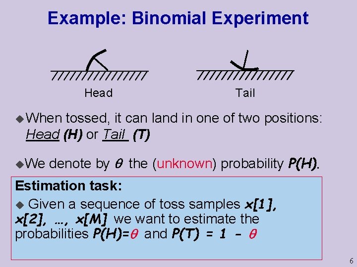
Example: Binomial Experiment Head Tail u When tossed, it can land in one of two positions: Head (H) or Tail (T) u. We denote by the (unknown) probability P(H). Estimation task: u Given a sequence of toss samples x[1], x[2], …, x[M] we want to estimate the probabilities P(H)= and P(T) = 1 - 6
![Statistical Parameter Fitting restement u Consider instances x1 x2 xM such that l Statistical Parameter Fitting (restement) u Consider instances x[1], x[2], …, x[M] such that l](https://slidetodoc.com/presentation_image_h/8c37160747cbd8dec07efbc4ad4128de/image-7.jpg)
Statistical Parameter Fitting (restement) u Consider instances x[1], x[2], …, x[M] such that l l l u The set of values that x can take is known i. i. d. Each is sampled from the same distribution Samples (why? ? ) Each sampled independently of the rest The task is to find a vector of parameters that have generated the given data. This vector parameter can be used to predict future data. 7

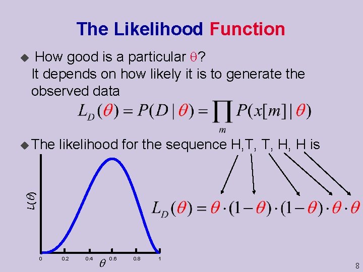
The Likelihood Function u How good is a particular ? It depends on how likely it is to generate the observed data likelihood for the sequence H, T, T, H, H is L( ) u The 0 0. 2 0. 4 0. 6 0. 8 1 8

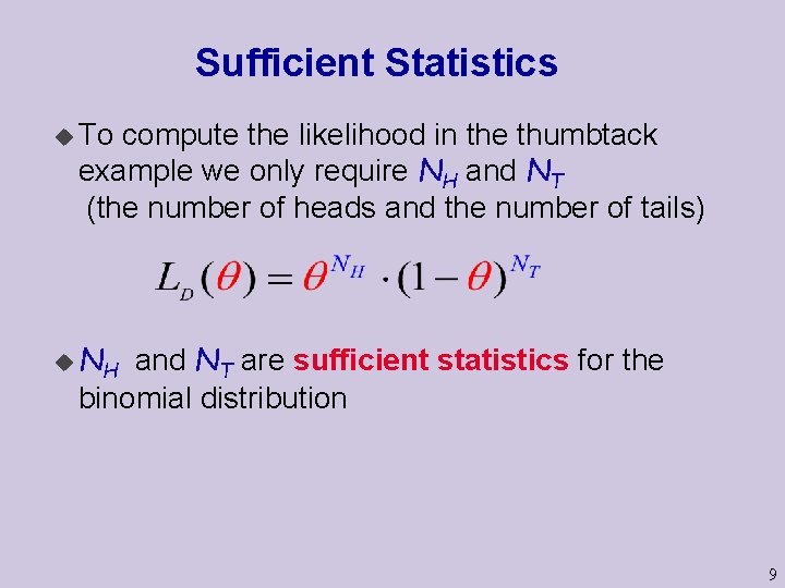
Sufficient Statistics u To compute the likelihood in the thumbtack example we only require NH and NT (the number of heads and the number of tails) u NH and NT are sufficient statistics for the binomial distribution 9

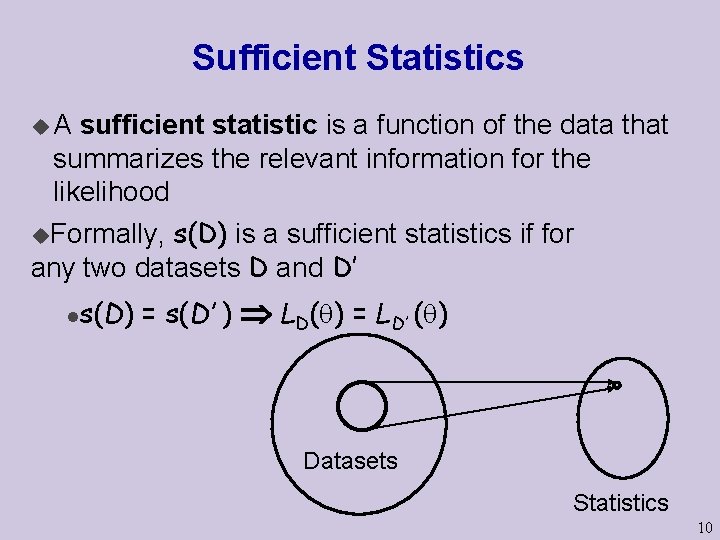
Sufficient Statistics u. A sufficient statistic is a function of the data that summarizes the relevant information for the likelihood s(D) is a sufficient statistics if for any two datasets D and D’ u. Formally, l s(D) = s(D’ ) LD( ) = LD’ ( ) Datasets Statistics 10

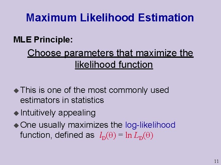
Maximum Likelihood Estimation MLE Principle: Choose parameters that maximize the likelihood function u This is one of the most commonly used estimators in statistics u Intuitively appealing u One usually maximizes the log-likelihood function, defined as l. D( ) = ln LD( ) 11

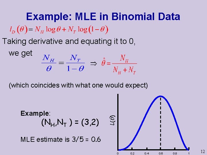
Example: MLE in Binomial Data Taking derivative and equating it to 0, we get Example: (NH, NT ) = (3, 2) L( ) (which coincides with what one would expect) MLE estimate is 3/5 = 0. 6 0 0. 2 0. 4 0. 6 0. 8 1 12

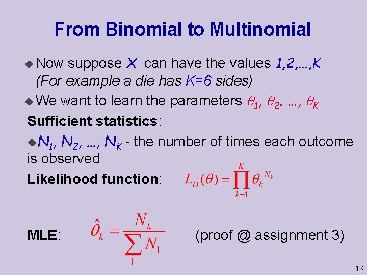
From Binomial to Multinomial suppose X can have the values 1, 2, …, K (For example a die has K=6 sides) u We want to learn the parameters 1, 2. …, K Sufficient statistics: u. N 1, N 2, …, NK - the number of times each outcome is observed Likelihood function: u Now MLE: (proof @ assignment 3) 13

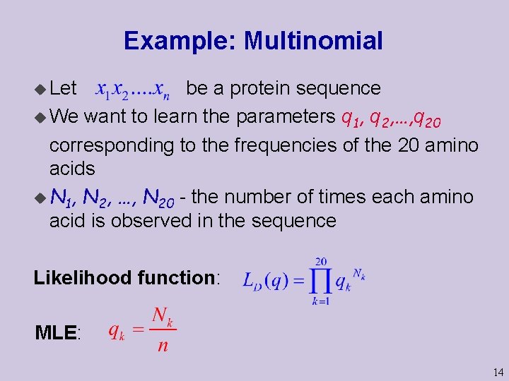
Example: Multinomial u Let be a protein sequence u We want to learn the parameters q 1, q 2, …, q 20 corresponding to the frequencies of the 20 amino acids u N 1, N 2, …, N 20 - the number of times each amino acid is observed in the sequence Likelihood function: MLE: 14

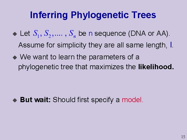
Inferring Phylogenetic Trees u Let be n sequence (DNA or AA). Assume for simplicity they are all same length, l. u u We want to learn the parameters of a phylogenetic tree that maximizes the likelihood. But wait: Should first specify a model. 15

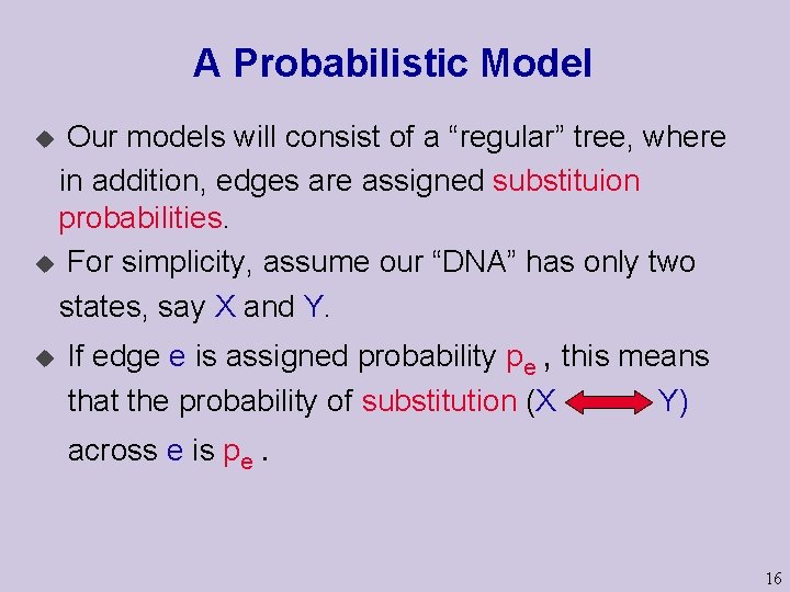
A Probabilistic Model Our models will consist of a “regular” tree, where in addition, edges are assigned substituion probabilities. u For simplicity, assume our “DNA” has only two states, say X and Y. u u If edge e is assigned probability pe , this means that the probability of substitution (X Y) across e is pe. 16

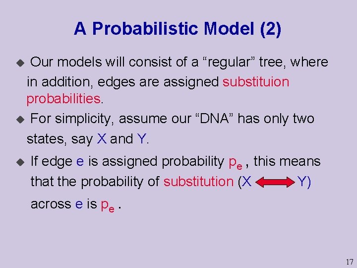
A Probabilistic Model (2) Our models will consist of a “regular” tree, where in addition, edges are assigned substituion probabilities. u For simplicity, assume our “DNA” has only two states, say X and Y. u u If edge e is assigned probability pe , this means that the probability of substitution (X Y) across e is pe. 17

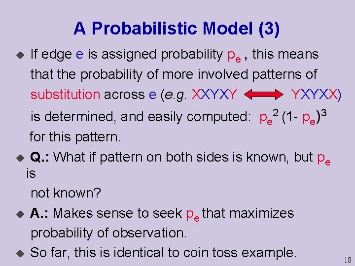
A Probabilistic Model (3) u If edge e is assigned probability pe , this means that the probability of more involved patterns of substitution across e (e. g. XXYXY YXYXX) is determined, and easily computed: pe 2 (1 - pe)3 for this pattern. u Q. : What if pattern on both sides is known, but pe is not known? u A. : Makes sense to seek pe that maximizes probability of observation. u So far, this is identical to coin toss example. 18

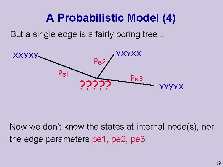
A Probabilistic Model (4) But a single edge is a fairly boring tree… XXYXY pe 1 pe 2 ? ? ? YXYXX pe 3 YYYYX Now we don’t know the states at internal node(s), nor the edge parameters pe 1, pe 2, pe 3 19

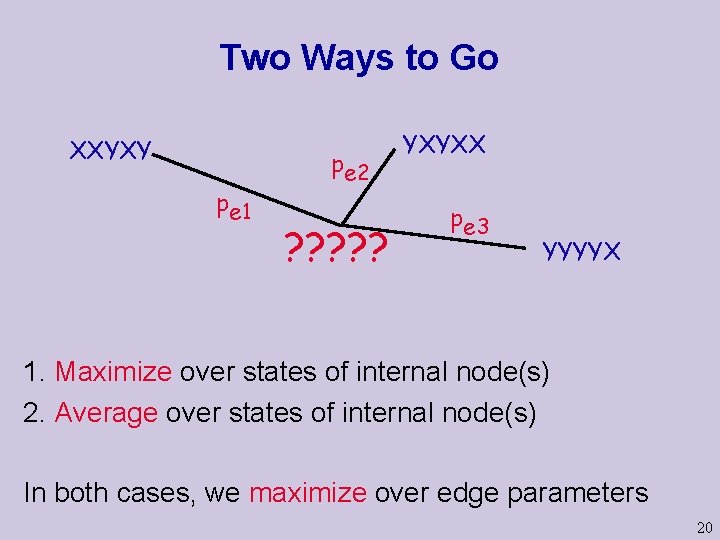
Two Ways to Go XXYXY pe 1 pe 2 ? ? ? YXYXX pe 3 YYYYX 1. Maximize over states of internal node(s) 2. Average over states of internal node(s) In both cases, we maximize over edge parameters 20

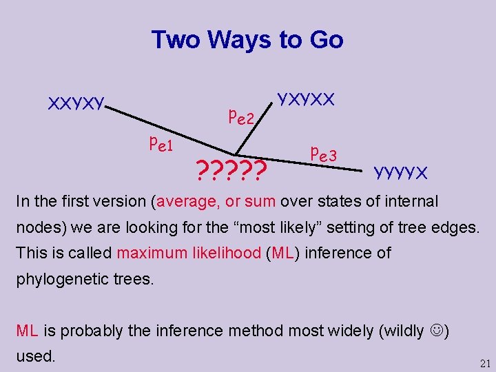
Two Ways to Go XXYXY pe 1 pe 2 ? ? ? YXYXX pe 3 YYYYX In the first version (average, or sum over states of internal nodes) we are looking for the “most likely” setting of tree edges. This is called maximum likelihood (ML) inference of phylogenetic trees. ML is probably the inference method most widely (wildly ) used. 21

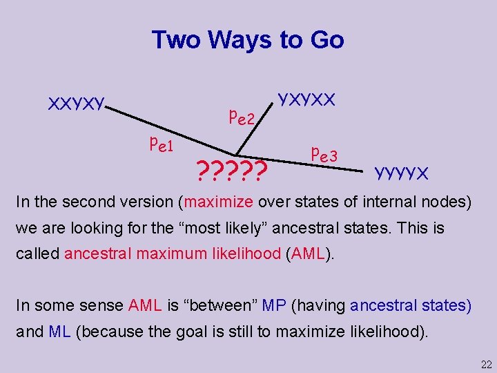
Two Ways to Go XXYXY pe 1 pe 2 ? ? ? YXYXX pe 3 YYYYX In the second version (maximize over states of internal nodes) we are looking for the “most likely” ancestral states. This is called ancestral maximum likelihood (AML). In some sense AML is “between” MP (having ancestral states) and ML (because the goal is still to maximize likelihood). 22

bust or a break.