Chapter 8 Profit Maximization and Competitive Supply Chapter

 Price taking – 短期 (Product")
 = Total Revenue -")
 R(q) Slope of R(q) =")
 Cost, Revenue, Profit $ (per year) Total Cost Slope of C(q) =")
與C(q) n 當產量是在 0 至 q 0: n C(q)>R(q)")
與C(q) n 問題: 為何產量 為零時, 利潤是 負的? Cost, Revenue,")
與C(q) n 產量在: q 0 - q* n R(q)>C(q) n")
與C(q) n 產量: q* Cost, Revenue, Profit $ (per year)")
與C(q) q*: n R(q)> C(q) n 產量超過 Cost, Revenue, Profit")
 C(q) A n")


 50 40 Lost profit for")
")


 1400 Observations • Price between $1140 & $1300: q")
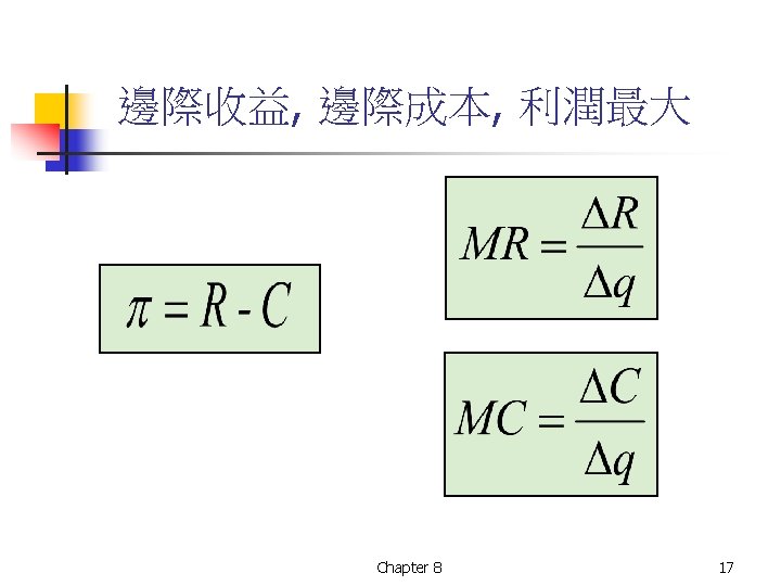
 MR = MC 決定 利潤最大的產量, 只要變動成本能賺回來就好 MC")

 S = MC above AVC MC P 2 ATC")
 MC 2 Savings to the firm from reducing output")
 27 提煉石化產品SMC 隨產量有階段變化, SMC 因提煉技術不同 26 產量多少? 當 P")

 Country Annual Production (thousand metric tons) Australia Canada Chile Indonesia Peru Poland")
 Country Annual Production (thousand metric tons) Australia Canada Chile Indonesia Peru Poland")
 0. 90 MCPo 0. 80 MCCa 0. 70 MCA")
 Producer Surplus MC 此例中, q* MC =")

 S 市場(產業)生產者剩餘 是價格與供給線所夾面積 P* Producer Surplus D")
 n 長期, 任何要素數量均可變, 包括規模 n 假設自由進出")
 長期, 規模擴大, 產量增加到 q 3. 長期利潤 EFGD")
 LMC LAC")


 MC = MR 2) P = LAC n 沒有進入或退出的動機 n")


 經濟利潤 新廠加入 $ per unit of output MC AC $ per")
 $ per unit of output SMC 2 SMC 1 LAC 2")
 $ per unit of output 因為要素價格下跌 產業長期均衡價跌 $ per unit of")
 S 2 = S 1 +")

- Slides: 70
Chapter 8 Profit Maximization and Competitive Supply 競爭市場的均衡與供給 Chapter 8
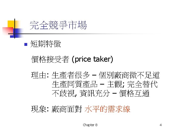
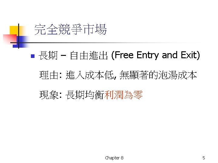
8. 1 完全競爭市場 Perfectly Competitive Markets n 特徵 1) Price taking – 短期 (Product homogeneity) 2) Free entry and exit – 長期 Chapter 8 3
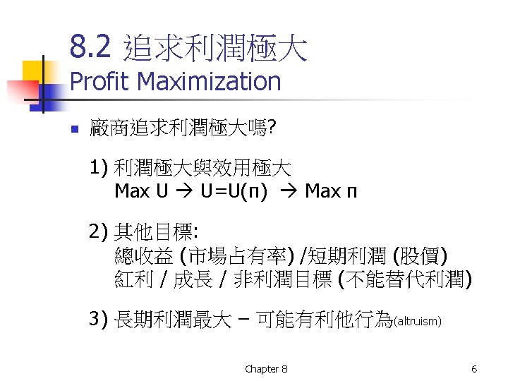
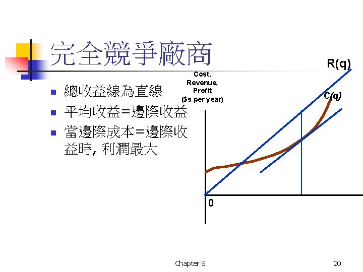
8. 3 邊際收益, 邊際成本, 利潤最大 n 利潤 Profit ( ) = Total Revenue - Total Cost Chapter 8 7
短期利潤最大 Total Revenue Cost, Revenue, Profit ($s per year) R(q) Slope of R(q) = MR 0 Output (units per year) Chapter 8 8
短期利潤最大 C(q) Cost, Revenue, Profit $ (per year) Total Cost Slope of C(q) = MC 為何產量為零時, 成本大於零? 0 Output (units per year) Chapter 8 9
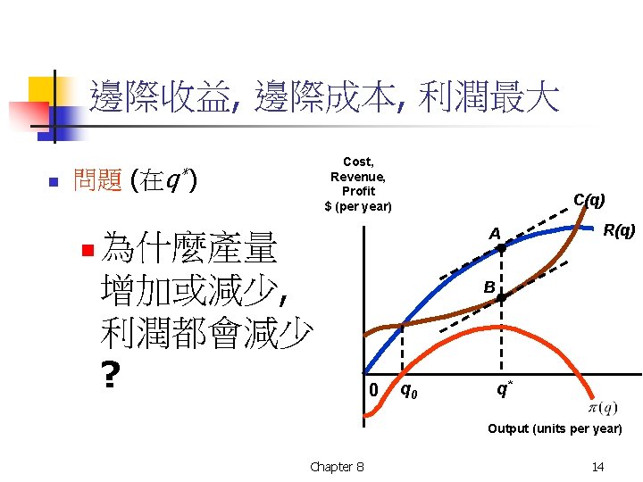
邊際收益, 邊際成本, 利潤最大 n 比較 R(q)與C(q) n 當產量是在 0 至 q 0: n C(q)>R(q) n n n Cost, Revenue, Profit ($s per year) C(q) A Negative profit FC + VC > R(q) B MR > MC n 產量增加 利潤提高 0 q* Output (units per year) Chapter 8 10
邊際收益, 邊際成本, 利潤最大 n 比較 R(q)與C(q) n 問題: 為何產量 為零時, 利潤是 負的? Cost, Revenue, Profit $ (per year) C(q) A R(q) B 0 q* Output (units per year) Chapter 8 11
邊際收益, 邊際成本, 利潤最大 n 比較R(q)與C(q) n 產量在: q 0 - q* n R(q)>C(q) n MR > MC Cost, Revenue, Profit $ (per year) C(q) A R(q) B 產量增加 利潤提高 0 q* Output (units per year) Chapter 8 12
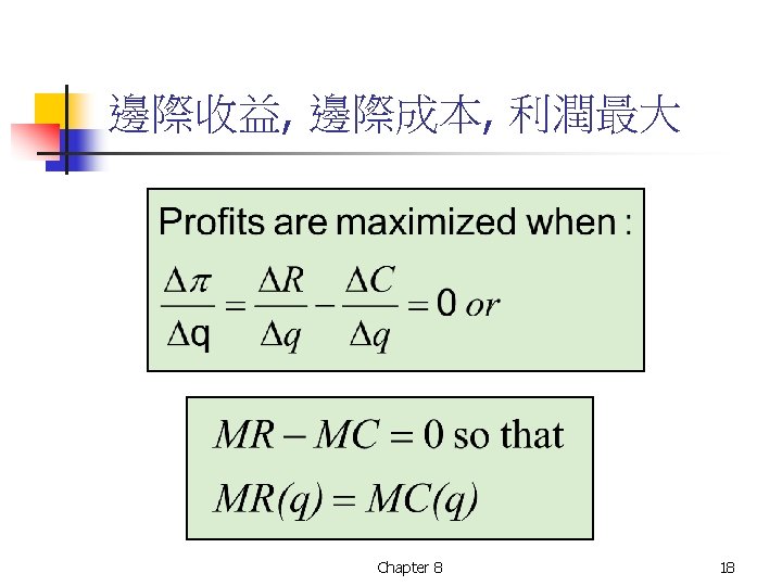
邊際收益, 邊際成本, 利潤最大 n 比較R(q)與C(q) n 產量: q* Cost, Revenue, Profit $ (per year) C(q) A R(q)>C(q) n MR = MC n Profit is maximized n R(q) B 0 q* Output (units per year) Chapter 8 13
邊際收益, 邊際成本, 利潤最大 n 比較R(q)與C(q) q*: n R(q)> C(q) n 產量超過 Cost, Revenue, Profit $ (per year) C(q) A R(q) B MC > MR n Profit is decreasing n 0 q* Output (units per year) Chapter 8 15
邊際收益, 邊際成本, 利潤最大 n 因此: Cost, Revenue, Profit $ (per year) C(q) A n 利潤最大時, 是在: MC = MR R(q) B 0 q* Output (units per year) Chapter 8 16
競爭市場的需求線 Price $ per bushel Firm $4 d Industry $4 D 100 200 Output (bushels) Chapter 8 100 Output (millions of bushels) 21
競爭廠商, 短期均衡, 有利潤 MC Price 60 ($ per unit) 50 40 Lost profit for qq < q * A D Lost profit for q 2 > q * ATC C B 30 AVC At q*: MR = MC and P > ATC q 1 : MR > MC and q 2: MC > MR 20 and q 0: MC = MR but MC falling 10 0 AR=MR=P 1 q 0 2 3 4 5 6 Chapter 8 7 q 1 8 q* 9 q 2 10 11 Output 24
A Competitive Firm – Positive Profits Price 50 40 Profit per unit = PAC(q) = A to B MC Total Profit = ABCD A D AR=MR=P ATC 30 C Profits are determined by output per unit times quantity AVC B 20 10 0 1 2 3 4 5 6 Chapter 8 7 q 1 8 q* 9 q 2 10 11 Output 25
A Competitive Firm – Losses MC Price ATC B C D A q *: 在 MR = MC 但 P < ATC 損失 (P-AC) x q* 或 ABCD P = MR AVC q* Chapter 8 Output 26
煉銅廠的短期產出 Cost (dollars per item) 1400 Observations • Price between $1140 & $1300: q = 600 • Price > $1300: q = 900 • Price < $1140: q = 0 P 2 1300 P 1 1200 Question Should the firm stay in business when P < $1140? 1140 1100 0 300 600 Chapter 8 900 Output (tons per day) 28
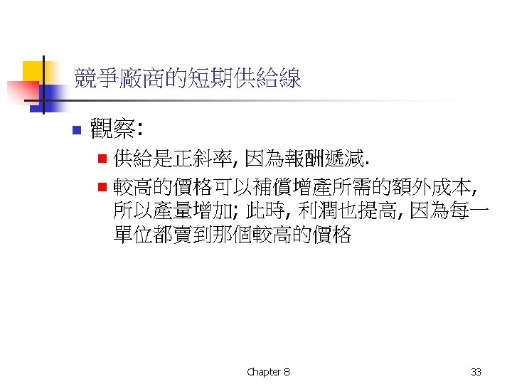
8. 5 競爭廠商的短期供給線 Price ($ per unit) MR = MC 決定 利潤最大的產量, 只要變動成本能賺回來就好 MC P 2 ATC P 1 AVC What happens if P < AVC? P = AVC q 1 Chapter 8 q 2 Output 30
競爭廠商的短期供給線 n Observations: P = MR n MR = MC n P = MC n n 供給就是價格與供給量的關係. 因此: If P = P 1, then q = q 1 n If P = P 2, then q = q 2 n Chapter 8 31
競爭廠商的短期供給線 Price ($ per unit) S = MC above AVC MC P 2 ATC P 1 AVC P = AVC Shut-down q 1 Chapter 8 q 2 Output 32
要素價格改變 Price ($ per unit) MC 2 Savings to the firm from reducing output 要素成本增加, MC 升到 MC 2 產量 q 減至 q 2. MC 1 $5 q 2 Chapter 8 q 1 Output 35
石化產品的短期生產 Cost ($ per barrel) 27 提煉石化產品SMC 隨產量有階段變化, SMC 因提煉技術不同 26 產量多少? 當 P = $23? P = $24 -$25? 25 24 23 8, 000 9, 000 10, 000 Chapter 8 11, 000 Output (barrels/day) 36
市場短期供給線 MC 1 $ per unit MC 2 MC 3 S 水平加線 P 3 P 2 P 1 2 4 5 7 8 10 Chapter 8 15 Q 21 38
世界銅產業 (1999) Country Annual Production (thousand metric tons) Australia Canada Chile Indonesia Peru Poland Russia United States Zambia 600 710 3660 750 420 450 1850 280 Chapter 8 Marginal Cost (dollars/pound) 0. 65 0. 75 0. 50 0. 55 0. 70 0. 80 0. 50 0. 70 0. 55 39
世界銅產業 (2001) Country Annual Production (thousand metric tons) Australia Canada Chile Indonesia Peru Poland Russia United States Zambia 900 620 4650 1080 560 450 550 1340 320 Chapter 8 Marginal Cost (dollars/pound) 0. 65 0. 75 0. 50 0. 55 0. 70 0. 80 0. 50 0. 70 0. 55 40
銅的短期世界供給 Price ($ per pound) 0. 90 MCPo 0. 80 MCCa 0. 70 MCA 0. 60 MCJ, MCZ MCC, MCR 0. 50 0. 40 MCP, MCUS 0 2000 4000 6000 8000 10000 Production (thousand metric tons) Chapter 8 41
生產者剩餘 Price ($ per unit of output) Producer Surplus MC 此例中, q* MC = MR. 在 0 與 q* 之間, 每一單位都是MR > MC AVC B A D 0 P C q* Chapter 8 另一種算法: TVC=ODCq*. TR=OABq*. PS=ABCD. Output 43
短期市場供給線 n Producer Surplus in the Short-Run 利潤 = π = TR – TVC – TFC 書上: 利潤 = π = R – VC – FC Chapter 8 44
市場的生產者剩餘 Price ($ per unit of output) S 市場(產業)生產者剩餘 是價格與供給線所夾面積 P* Producer Surplus D Q* Chapter 8 Output 46
8. 7長期均衡產量 (Choosing Output in the Long Run) n 長期, 任何要素數量均可變, 包括規模 n 假設自由進出 (free entry and free exit). Chapter 8 47
長期均衡產量 Price ($ per unit of output) 長期, 規模擴大, 產量增加到 q 3. 長期利潤 EFGD > 短期的ABCD. LMC LAC SMC D $40 SAC A C G E B P = MR F $30 短期受制於固定要素 在 P = $40 > ATC. 利潤為 ABCD. q 1 q 2 Chapter 8 q 3 Output 48
長期均衡產量 問題: 如果因為產量增加, 價格降到 $30, 廠商仍有利潤嗎? Price ($ per unit of output) LMC LAC SMC D $40 SAC A C G E B P = MR F $30 q 1 q 2 Chapter 8 q 3 Output 49
長期 –進出自由 • 利潤引誘新廠 供給增加一直到利潤為零 $ per unit of output Firm Industry S 1 LMC $40 LAC $30 P 1 S 2 P 2 D q 2 Q 1 Output Chapter 8 Q 2 Output 51
長期的競爭均衡 – 虧損 • 虧損會使廠商退出, 供給減少, 恢復利潤到零 $ per unit of output Firm LMC $ per unit of output LAC $30 P 2 $20 P 1 Industry S 2 S 1 D q 2 Output Chapter 8 Q 2 Q 1 Output 52
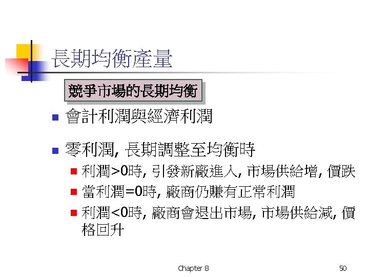
長期均衡產量 n 長期競爭均衡 1) MC = MR 2) P = LAC n 沒有進入或退出的動機 n Profit = 0 3) Equilibrium Market Price Chapter 8 53
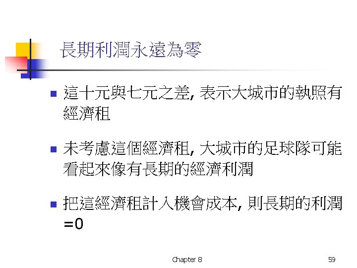
長期利潤永遠為零 Ticket Price LMC LAC 中型城市的 美式足球隊 門票 =$7 利潤為零 $7 1. 0 Chapter 8 Season Tickets Sales (millions) 57
長期利潤永遠為零 Ticket Price LAC Economic Rent LMC $10 $7 同一隊在大城市 可賣門票到 $10 1. 3 Chapter 8 Season Tickets Sales (millions) 58
成本不變產業 (Constant-Cost Industry) 經濟利潤 新廠加入 $ per unit of output MC AC $ per unit of output P 2 Q 1 增至Q 2 長期供給線 = SL = LRAC. S 1 S 2 C P 2 A P 1 B SL P 1 D 1 q 2 Q 1 Output Chapter 8 Q 2 D 2 Output 61
成本遞增產業 (Increasing-Cost Industry) $ per unit of output SMC 2 SMC 1 LAC 2 LAC 1 P 2 $ per unit of output 產業產量增加, 要素漲價 導至長期均衡價格提高 S 1 S 2 P 3 P 1 P 1 B A D 1 q 2 SL Q 1 Output Chapter 8 Q 2 Q 3 D 1 Output 62
成本遞減產業 (Decreasing-Cost Industry) $ per unit of output 因為要素價格下跌 產業長期均衡價跌 $ per unit of output SMC 1 S 2 SMC 2 LAC 1 P 2 LAC 2 P 1 P 3 A B SL D 1 q 2 Q 1 Q 2 Output Chapter 8 Q 3 D 2 Output 63
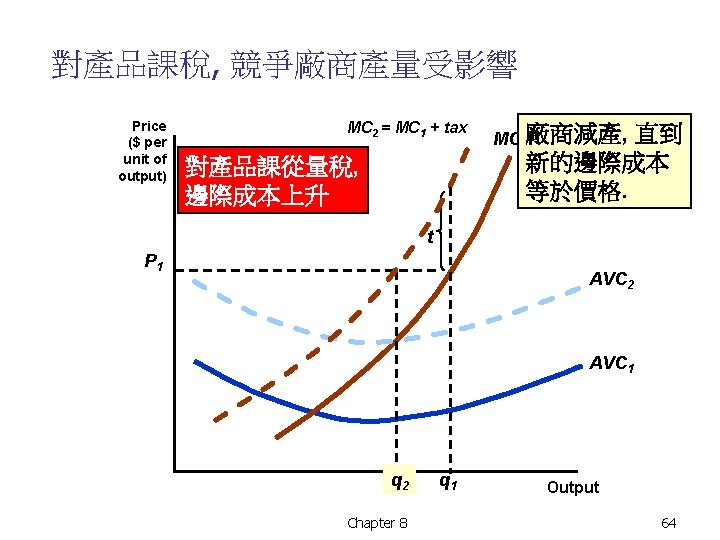
對產品課稅, 產業的產量受影響 Price ($ per unit of output) S 2 = S 1 + t S 1 t P 2 S 1 移到 S 2 產量減到 Q 2 價格漲到 P 2. P 1 D Q 2 Q 1 Chapter 8 Output 65
End of Chapter 8 Profit Maximization and Competitive Supply Chapter 8