Chapter 9 Linear Programming The Simplex Method To

Chapter 9 Linear Programming: The Simplex Method To accompany Quantitative Analysis for Management, Tenth Edition, by Render, Stair, and Hanna Power Point slides created by Jeff Heyl © 2008 Prentice-Hall, Inc. © 2009 Prentice-Hall, Inc.

Learning Objectives After completing this chapter, students will be able to: 1. Convert LP constraints to equalities with slack, 2. 3. 4. 5. 6. surplus, and artificial variables Set up and solve LP problems with simplex tableaus Interpret the meaning of every number in a simplex tableau Recognize special cases such as infeasibility, unboundedness, and degeneracy Use the simplex tables to conduct sensitivity analysis Construct the dual problem from the primal problem © 2009 Prentice-Hall, Inc. 9– 2

Chapter Outline 9. 1 Introduction 9. 2 How to Set Up the Initial Simplex Solution 9. 3 Simplex Solution Procedures 9. 4 The Second Simplex Tableau 9. 5 Developing the Third Tableau 9. 6 Review of Procedures for Solving LP Maximization Problems 9. 7 Surplus and Artificial Variables © 2009 Prentice-Hall, Inc. 9– 3

Chapter Outline 9. 8 9. 9 9. 10 9. 11 9. 12 9. 13 Solving Minimization Problems Review of Procedures for Solving LP Minimization Problems Special Cases Sensitivity Analysis with the Simplex Tableau The Dual Karmarkar’s Algorithm © 2009 Prentice-Hall, Inc. 9– 4

Introduction n With only two decision variables it is possible to n n n use graphical methods to solve LP problems But most real life LP problems are too complex for simple graphical procedures We need a more powerful procedure called the simplex method The simplex method examines the corner points in a systematic fashion using basic algebraic concepts It does this in an iterative manner until an optimal solution is found Each iteration moves us closer to the optimal solution © 2009 Prentice-Hall, Inc. 9– 5

Introduction n Why should we study the simplex method? n It is important to understand the ideas used to produce solutions n It provides the optimal solution to the decision variables and the maximum profit (or minimum cost) n It also provides important economic information n To be able to use computers successfully and to interpret LP computer printouts, we need to know what the simplex method is doing and why © 2009 Prentice-Hall, Inc. 9– 6

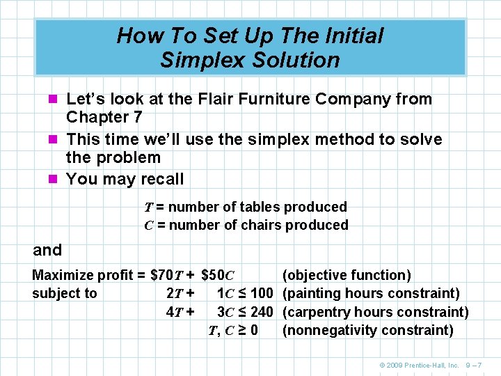
How To Set Up The Initial Simplex Solution n Let’s look at the Flair Furniture Company from Chapter 7 n This time we’ll use the simplex method to solve the problem n You may recall T = number of tables produced C = number of chairs produced and Maximize profit = $70 T + $50 C subject to 2 T + 1 C ≤ 100 4 T + 3 C ≤ 240 T, C ≥ 0 (objective function) (painting hours constraint) (carpentry hours constraint) (nonnegativity constraint) © 2009 Prentice-Hall, Inc. 9– 7

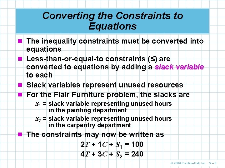
Converting the Constraints to Equations n The inequality constraints must be converted into equations n Less-than-or-equal-to constraints (≤) are converted to equations by adding a slack variable to each n Slack variables represent unused resources n For the Flair Furniture problem, the slacks are S 1 = slack variable representing unused hours in the painting department S 2 = slack variable representing unused hours in the carpentry department n The constraints may now be written as 2 T + 1 C + S 1 = 100 4 T + 3 C + S 2 = 240 © 2009 Prentice-Hall, Inc. 9– 8

Converting the Constraints to Equations n If the optimal solution uses less than the available amount of a resource, the unused resource is slack n For example, if Flair produces T = 40 tables and C = 10 chairs, the painting constraint will be 2 T + 1 C + S 1 = 100 2(40) +1(10) + S 1 = 100 S 1 = 10 n There will be 10 hours of slack, or unused painting capacity © 2009 Prentice-Hall, Inc. 9– 9

Converting the Constraints to Equations n Each slack variable must appear in every constraint equation n Slack variables not actually needed for an equation have a coefficient of 0 n So 2 T + 1 C + 1 S 1 + 0 S 2 = 100 4 T + 3 C +0 S 1 + 1 S 2 = 240 T, C, S 1, S 2 ≥ 0 n The objective function becomes Maximize profit = $70 T + $50 C + $0 S 1 + $0 S 2 © 2009 Prentice-Hall, Inc. 9 – 10

Finding an Initial Solution Algebraically n There are now two equations and four variables n When there are more unknowns than equations, you have to set some of the variables equal to 0 and solve for the others n In this example, two variables must be set to 0 so we can solve for the other two n A solution found in this manner is called a basic feasible solution © 2009 Prentice-Hall, Inc. 9 – 11

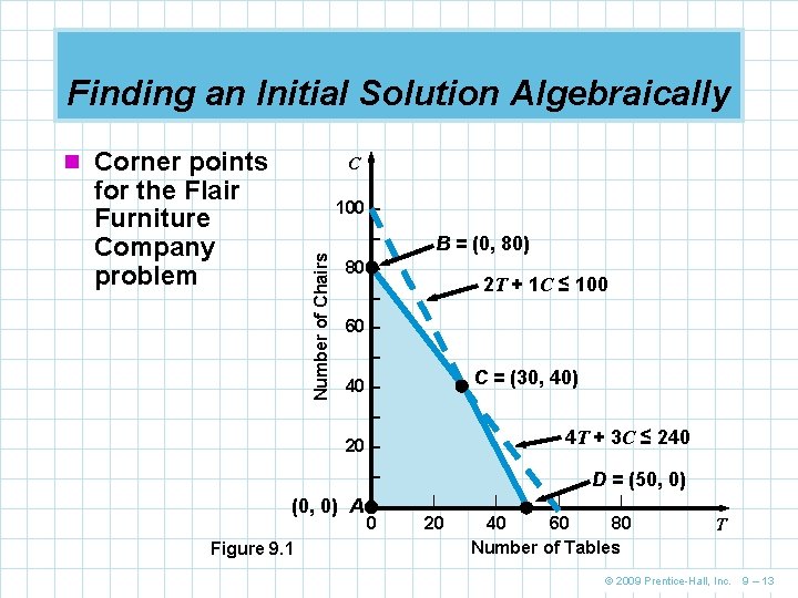
Finding an Initial Solution Algebraically n The simplex method starts with an initial feasible n n solution where all real variables are set to 0 While this is not an exciting solution, it is a corner point solution Starting from this point, the simplex method will move to the corner point that yields the most improved profit It repeats the process until it can further improve the solution On the following graph, the simplex method starts at point A and then moves to B and finally to C, the optimal solution © 2009 Prentice-Hall, Inc. 9 – 12

Finding an Initial Solution Algebraically n Corner points C for the Flair Furniture Company problem 100 – Number of Chairs – B = (0, 80) 80 – 2 T + 1 C ≤ 100 – 60 – – C = (30, 40) 40 – – 20 – 4 T + 3 C ≤ 240 – D = (50, 0) (0, 0) A |– 0 Figure 9. 1 | 20 | | | 40 60 80 Number of Tables T © 2009 Prentice-Hall, Inc. 9 – 13

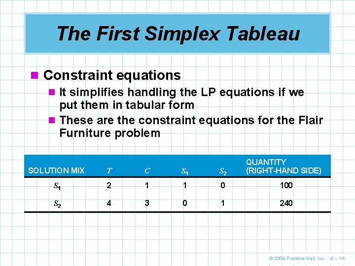
The First Simplex Tableau n Constraint equations n It simplifies handling the LP equations if we put them in tabular form n These are the constraint equations for the Flair Furniture problem QUANTITY (RIGHT-HAND SIDE) SOLUTION MIX T C S 1 S 2 S 1 2 1 1 0 100 S 2 4 3 0 1 240 © 2009 Prentice-Hall, Inc. 9 – 14

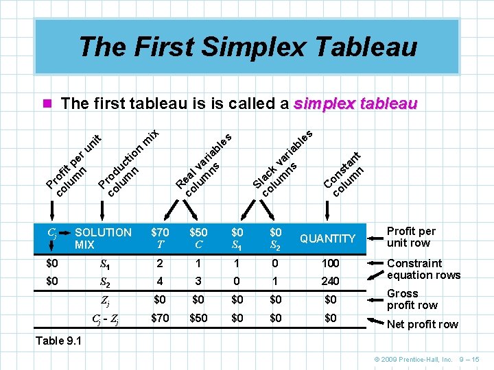
The First Simplex Tableau s C co on lu sta m n n t S co lac lu k v m a ns ria b le es R co ea lu l va m r ns iab l m ix P co rod lu uc m ti n on P co rof lu it p m e n ru ni t n The first tableau is is called a simplex tableau Cj SOLUTION MIX $70 T $50 C $0 S 1 $0 S 2 QUANTITY $0 S 1 2 1 1 0 100 $0 S 2 4 3 0 1 240 Zj $0 $0 $0 Cj - Zj $70 $50 $0 $0 $0 Profit per unit row Constraint equation rows Gross profit row Net profit row Table 9. 1 © 2009 Prentice-Hall, Inc. 9 – 15

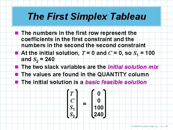
The First Simplex Tableau n The numbers in the first row represent the n n coefficients in the first constraint and the numbers in the second constraint At the initial solution, T = 0 and C = 0, so S 1 = 100 and S 2 = 240 The two slack variables are the initial solution mix The values are found in the QUANTITY column The initial solution is a basic feasible solution T C S 1 S 2 = 0 0 100 240 © 2009 Prentice-Hall, Inc. 9 – 16

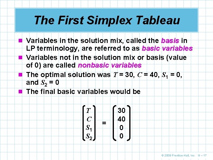
The First Simplex Tableau n Variables in the solution mix, called the basis in LP terminology, are referred to as basic variables n Variables not in the solution mix or basis (value of 0) are called nonbasic variables n The optimal solution was T = 30, C = 40, S 1 = 0, and S 2 = 0 n The final basic variables would be T C S 1 S 2 = 30 40 0 0 © 2009 Prentice-Hall, Inc. 9 – 17

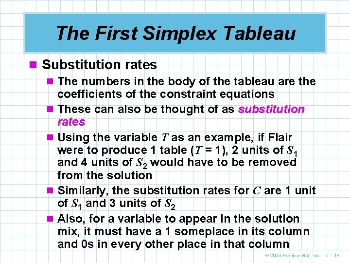
The First Simplex Tableau n Substitution rates n The numbers in the body of the tableau are the coefficients of the constraint equations n These can also be thought of as substitution rates n Using the variable T as an example, if Flair were to produce 1 table (T = 1), 2 units of S 1 and 4 units of S 2 would have to be removed from the solution n Similarly, the substitution rates for C are 1 unit of S 1 and 3 units of S 2 n Also, for a variable to appear in the solution mix, it must have a 1 someplace in its column and 0 s in every other place in that column © 2009 Prentice-Hall, Inc. 9 – 18

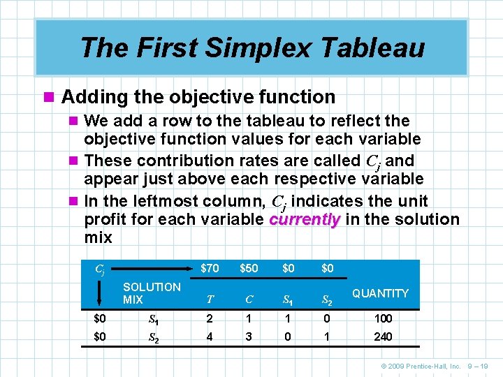
The First Simplex Tableau n Adding the objective function n We add a row to the tableau to reflect the objective function values for each variable n These contribution rates are called Cj and appear just above each respective variable n In the leftmost column, Cj indicates the unit profit for each variable currently in the solution mix $70 $50 $0 $0 SOLUTION MIX T C S 1 S 2 $0 S 1 2 1 1 0 100 $0 S 2 4 3 0 1 240 Cj QUANTITY © 2009 Prentice-Hall, Inc. 9 – 19

The First Simplex Tableau n The Zj and Cj – Zj rows n We can complete the initial tableau by adding two final rows n These rows provide important economic information including total profit and whether the current solution is optimal n We compute the Zj value by multiplying the contribution value of each number in a column by each number in that row and the jth column, and summing © 2009 Prentice-Hall, Inc. 9 – 20

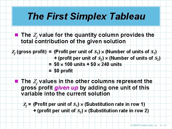
The First Simplex Tableau n The Zj value for the quantity column provides the total contribution of the given solution Zj (gross profit) = (Profit per unit of S 1) (Number of units of S 1) + (profit per unit of S 2) (Number of units of S 2) = $0 100 units + $0 240 units = $0 profit n The Zj values in the other columns represent the gross profit given up by adding one unit of this variable into the current solution Zj = (Profit per unit of S 1) (Substitution rate in row 1) + (profit per unit of S 2) (Substitution rate in row 2) © 2009 Prentice-Hall, Inc. 9 – 21

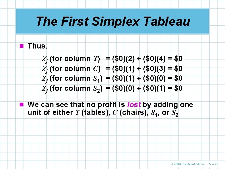
The First Simplex Tableau n Thus, Zj (for column T) Zj (for column C) Zj (for column S 1) Zj (for column S 2) = ($0)(2) + ($0)(4) = $0 = ($0)(1) + ($0)(3) = $0 = ($0)(1) + ($0)(0) = $0 = ($0)(0) + ($0)(1) = $0 n We can see that no profit is lost by adding one unit of either T (tables), C (chairs), S 1, or S 2 © 2009 Prentice-Hall, Inc. 9 – 22

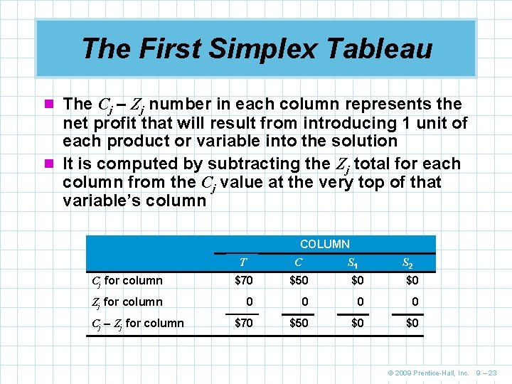
The First Simplex Tableau n The Cj – Zj number in each column represents the net profit that will result from introducing 1 unit of each product or variable into the solution n It is computed by subtracting the Zj total for each column from the Cj value at the very top of that variable’s column COLUMN T C Cj for column $70 Zj for column Cj – Zj for column S 1 S 2 $50 $0 $0 0 0 $70 $50 $0 $0 © 2009 Prentice-Hall, Inc. 9 – 23

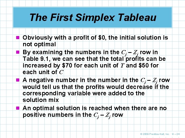
The First Simplex Tableau n Obviously with a profit of $0, the initial solution is not optimal n By examining the numbers in the Cj – Zj row in Table 9. 1, we can see that the total profits can be increased by $70 for each unit of T and $50 for each unit of C n A negative number in the Cj – Zj row would tell us that the profits would decrease if the corresponding variable were added to the solution mix n An optimal solution is reached when there are no positive numbers in the Cj – Zj row © 2009 Prentice-Hall, Inc. 9 – 24

Simplex Solution Procedures n After an initial tableau has been completed, we proceed through a series of five steps to compute all the numbers needed in the next tableau n The calculations are not difficult, but they are complex enough that even the smallest arithmetic error can produce a wrong answer © 2009 Prentice-Hall, Inc. 9 – 25

Five Steps of the Simplex Method for Maximization Problems 1. Determine the variable to enter the solution mix next. One way of doing this is by identifying the column, and hence the variable, with the largest positive number in the Cj - Zj row of the preceding tableau. The column identified in this step is called the pivot column 2. Determine which variable to replace. This is accomplished by dividing the quantity column by the corresponding number in the column selected in step 1. The row with the smallest nonnegative number calculated in this fashion will be replaced in the next tableau. This row is often referred to as the pivot row The number at the intersection of the pivot row and pivot column is the pivot number © 2009 Prentice-Hall, Inc. 9 – 26

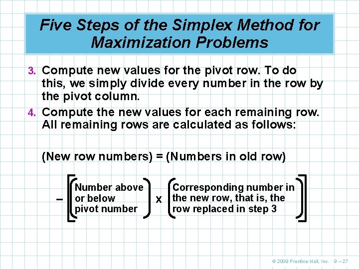
Five Steps of the Simplex Method for Maximization Problems 3. Compute new values for the pivot row. To do this, we simply divide every number in the row by the pivot column. 4. Compute the new values for each remaining row. All remaining rows are calculated as follows: (New row numbers) = (Numbers in old row) – Number above or below pivot number x Corresponding number in the new row, that is, the row replaced in step 3 © 2009 Prentice-Hall, Inc. 9 – 27

Five Steps of the Simplex Method for Maximization Problems 5. Compute the Zj and Cj - Zj rows, as demonstrated in the initial tableau. If all the numbers in the Cj - Zj row are 0 or negative, an optimal solution has been reached. If this is not the case, return to step 1. © 2009 Prentice-Hall, Inc. 9 – 28

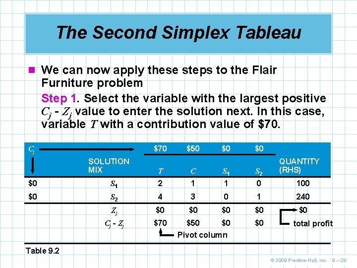
The Second Simplex Tableau n We can now apply these steps to the Flair Furniture problem Step 1. 1 Select the variable with the largest positive Cj - Zj value to enter the solution next. In this case, variable T with a contribution value of $70 Cj SOLUTION MIX $50 $0 $0 T C S 1 S 2 QUANTITY (RHS) $0 S 1 2 1 1 0 100 $0 S 2 4 3 0 1 240 Zj $0 $0 $0 Cj - Zj $70 $50 $0 Pivot column $0 total profit Table 9. 2 © 2009 Prentice-Hall, Inc. 9 – 29

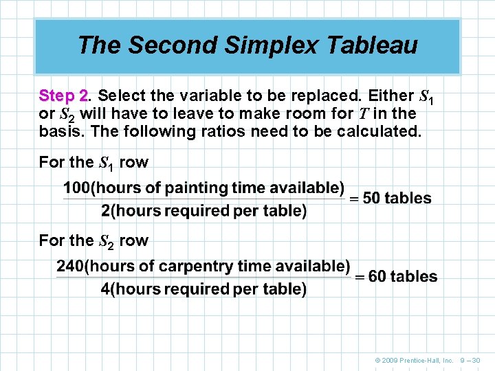
The Second Simplex Tableau Step 2. 2 Select the variable to be replaced. Either S 1 or S 2 will have to leave to make room for T in the basis. The following ratios need to be calculated. For the S 1 row For the S 2 row © 2009 Prentice-Hall, Inc. 9 – 30

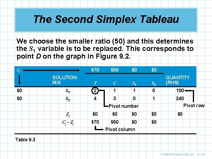
The Second Simplex Tableau We choose the smaller ratio (50) and this determines the S 1 variable is to be replaced. This corresponds to point D on the graph in Figure 9. 2. $70 Cj SOLUTION MIX $50 $0 $0 T C S 1 S 2 QUANTITY (RHS) $0 S 1 2 1 1 0 100 $0 S 2 4 3 0 1 240 Pivot row $0 Pivot number Zj $0 $0 Cj - Zj $70 $50 $0 $0 Pivot column Table 9. 3 © 2009 Prentice-Hall, Inc. 9 – 31

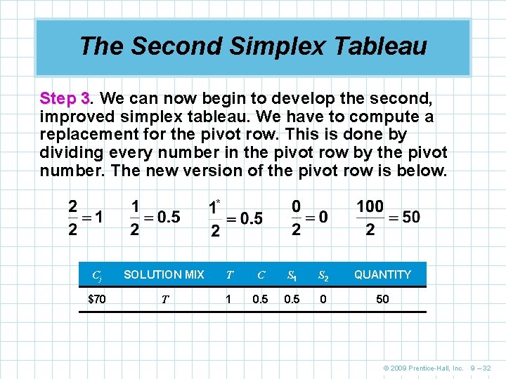
The Second Simplex Tableau Step 3. 3 We can now begin to develop the second, improved simplex tableau. We have to compute a replacement for the pivot row. This is done by dividing every number in the pivot row by the pivot number. The new version of the pivot row is below. Cj SOLUTION MIX T C S 1 S 2 QUANTITY $70 T 1 0. 5 0 50 © 2009 Prentice-Hall, Inc. 9 – 32

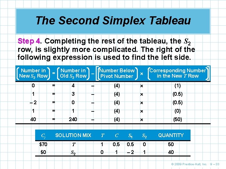
The Second Simplex Tableau Step 4. 4 Completing the rest of the tableau, the S 2 row, is slightly more complicated. The right of the following expression is used to find the left side. Number in = – New S 2 Row Old S 2 Row Number Below Pivot Number Corresponding Number in the New T Row 0 = 4 – (4) (1) 1 = 3 – (4) (0. 5) – 2 = 0 – (4) (0. 5) 1 = 1 – (4) (0) 40 = 240 – (4) (50) Cj SOLUTION MIX T C S 1 S 2 QUANTITY $70 T 1 0. 5 0 50 $0 S 2 0 1 – 2 1 40 © 2009 Prentice-Hall, Inc. 9 – 33

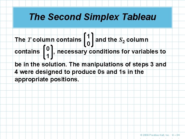
The Second Simplex Tableau 1 The T column contains and the S 2 column 0 contains 0 , necessary conditions for variables to 1 be in the solution. The manipulations of steps 3 and 4 were designed to produce 0 s and 1 s in the appropriate positions. © 2009 Prentice-Hall, Inc. 9 – 34

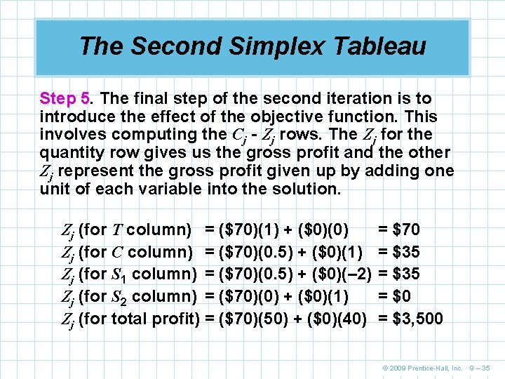
The Second Simplex Tableau Step 5. 5 The final step of the second iteration is to introduce the effect of the objective function. This involves computing the Cj - Zj rows. The Zj for the quantity row gives us the gross profit and the other Zj represent the gross profit given up by adding one unit of each variable into the solution. Zj (for T column) = ($70)(1) + ($0)(0) Zj (for C column) = ($70)(0. 5) + ($0)(1) Zj (for S 1 column) = ($70)(0. 5) + ($0)(– 2) Zj (for S 2 column) = ($70)(0) + ($0)(1) Zj (for total profit) = ($70)(50) + ($0)(40) = $70 = $35 = $0 = $3, 500 © 2009 Prentice-Hall, Inc. 9 – 35

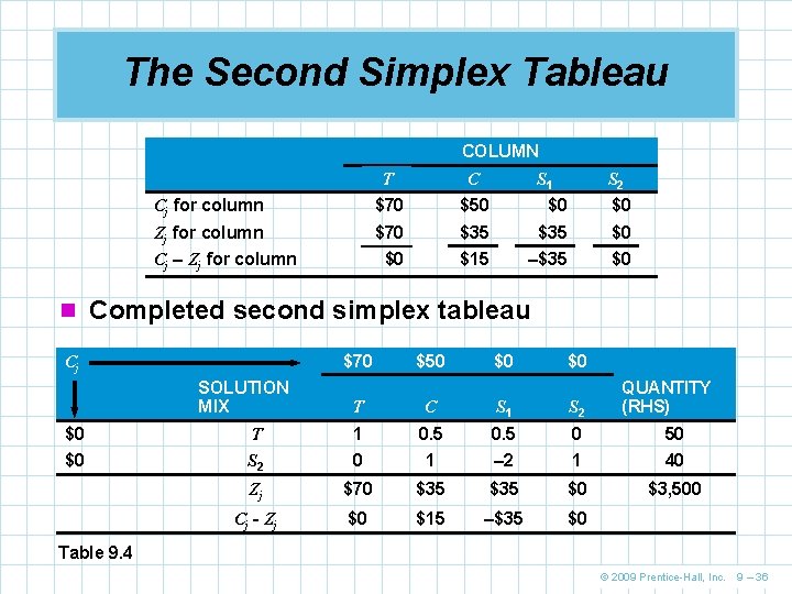
The Second Simplex Tableau COLUMN T C Cj for column $70 $50 $0 $0 Zj for column $70 $35 $0 $0 $15 –$35 $0 Cj – Zj for column S 1 S 2 n Completed second simplex tableau $70 Cj SOLUTION MIX $50 $0 $0 T C S 1 S 2 QUANTITY (RHS) $0 T 1 0. 5 0 50 $0 S 2 0 1 – 2 1 40 Zj $70 $35 $0 $3, 500 Cj - Zj $0 $15 –$35 $0 Table 9. 4 © 2009 Prentice-Hall, Inc. 9 – 36

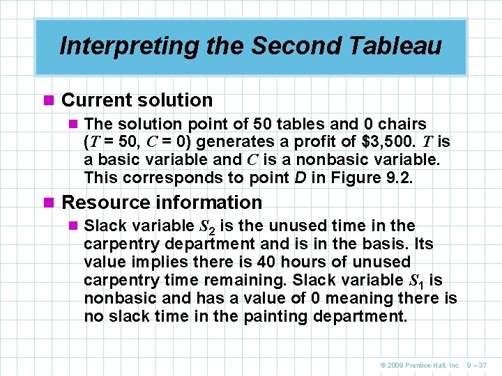
Interpreting the Second Tableau n Current solution n The solution point of 50 tables and 0 chairs (T = 50, C = 0) generates a profit of $3, 500. T is a basic variable and C is a nonbasic variable. This corresponds to point D in Figure 9. 2. n Resource information n Slack variable S 2 is the unused time in the carpentry department and is in the basis. Its value implies there is 40 hours of unused carpentry time remaining. Slack variable S 1 is nonbasic and has a value of 0 meaning there is no slack time in the painting department. © 2009 Prentice-Hall, Inc. 9 – 37

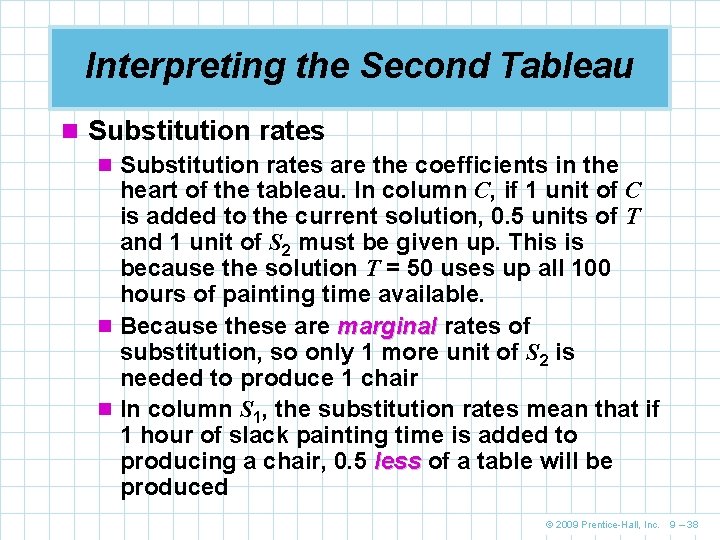
Interpreting the Second Tableau n Substitution rates are the coefficients in the heart of the tableau. In column C, if 1 unit of C is added to the current solution, 0. 5 units of T and 1 unit of S 2 must be given up. This is because the solution T = 50 uses up all 100 hours of painting time available. n Because these are marginal rates of substitution, so only 1 more unit of S 2 is needed to produce 1 chair n In column S 1, the substitution rates mean that if 1 hour of slack painting time is added to producing a chair, 0. 5 less of a table will be produced © 2009 Prentice-Hall, Inc. 9 – 38

Interpreting the Second Tableau n Net profit row n The Cj - Zj row is important for two reasons n First, it indicates whether the current solution is optimal n When there are no positive values in the bottom row, an optimal solution to a maximization LP has been reached n The second reason is that we use this row to determine which variable will enter the solution next © 2009 Prentice-Hall, Inc. 9 – 39

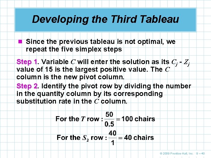
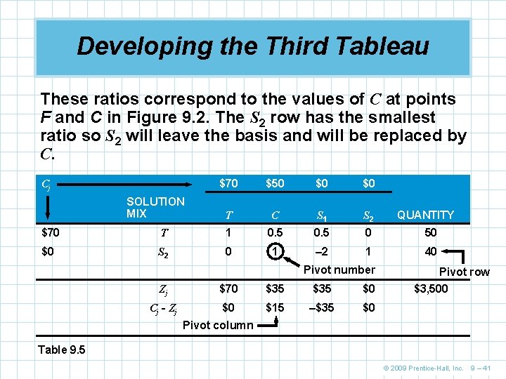
Developing the Third Tableau n Since the previous tableau is not optimal, we repeat the five simplex steps Step 1. 1 Variable C will enter the solution as its Cj - Zj value of 15 is the largest positive value. The C column is the new pivot column. Step 2. 2 Identify the pivot row by dividing the number in the quantity column by its corresponding substitution rate in the C column. © 2009 Prentice-Hall, Inc. 9 – 40

Developing the Third Tableau These ratios correspond to the values of C at points F and C in Figure 9. 2. The S 2 row has the smallest ratio so S 2 will leave the basis and will be replaced by C. Cj SOLUTION MIX $70 $50 $0 $0 T C S 1 S 2 QUANTITY $70 T 1 0. 5 0 50 $0 S 2 0 1 – 2 1 40 Pivot number Zj $70 $35 $0 Cj - Zj $0 $15 –$35 $0 Pivot row $3, 500 Pivot column Table 9. 5 © 2009 Prentice-Hall, Inc. 9 – 41

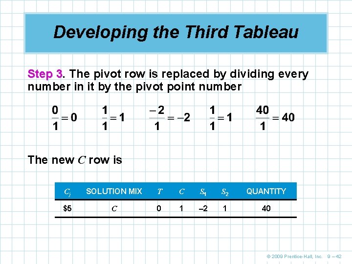
Developing the Third Tableau Step 3. 3 The pivot row is replaced by dividing every number in it by the pivot point number The new C row is Cj SOLUTION MIX T C S 1 S 2 QUANTITY $5 C 0 1 – 2 1 40 © 2009 Prentice-Hall, Inc. 9 – 42

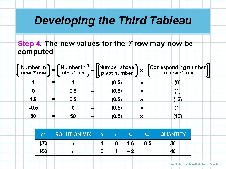
Developing the Third Tableau Step 4. 4 The new values for the T row may now be computed Number in new T row = Number in old T row – Number above pivot number Corresponding number in new C row 1 = 1 – (0. 5) (0) 0 = 0. 5 – (0. 5) (1) 1. 5 = 0. 5 – (0. 5) (– 2) – 0. 5 = 0 – (0. 5) (1) 30 = 50 – (0. 5) (40) Cj SOLUTION MIX T C S 1 S 2 QUANTITY $70 T 1 0 1. 5 – 0. 5 30 $50 C 0 1 – 2 1 40 © 2009 Prentice-Hall, Inc. 9 – 43

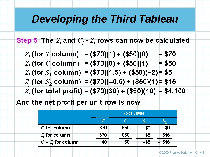
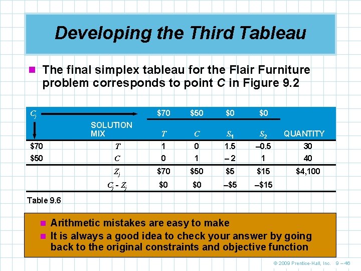
Developing the Third Tableau Step 5. 5 The Zj and Cj - Zj rows can now be calculated Zj (for T column) = ($70)(1) + ($50)(0) = $70 Zj (for C column) = ($70)(0) + ($50)(1) = $50 Zj (for S 1 column) = ($70)(1. 5) + ($50)(– 2)= $5 Zj (for S 2 column) = ($70)(– 0. 5) + ($50)(1)= $15 Zj (for total profit) = ($70)(30) + ($50)(40) = $4, 100 And the net profit per unit row is now COLUMN T C Cj for column $70 $50 $0 $0 Zj for column $70 $5 $15 $0 $0 –$5 – $15 Cj – Zj for column S 1 S 2 © 2009 Prentice-Hall, Inc. 9 – 44

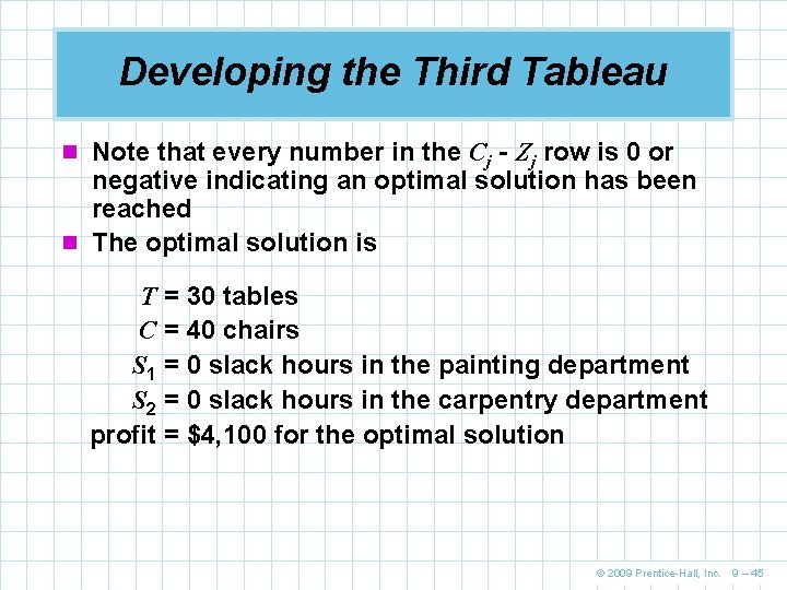
Developing the Third Tableau n Note that every number in the Cj - Zj row is 0 or negative indicating an optimal solution has been reached n The optimal solution is T = 30 tables C = 40 chairs S 1 = 0 slack hours in the painting department S 2 = 0 slack hours in the carpentry department profit = $4, 100 for the optimal solution © 2009 Prentice-Hall, Inc. 9 – 45

Developing the Third Tableau n The final simplex tableau for the Flair Furniture problem corresponds to point C in Figure 9. 2 Cj SOLUTION MIX $70 $50 $0 $0 T C S 1 S 2 QUANTITY $70 T 1 0 1. 5 – 0. 5 30 $50 C 0 1 – 2 1 40 Zj $70 $5 $15 $4, 100 Cj - Zj $0 $0 –$5 –$15 Table 9. 6 n Arithmetic mistakes are easy to make n It is always a good idea to check your answer by going back to the original constraints and objective function © 2009 Prentice-Hall, Inc. 9 – 46

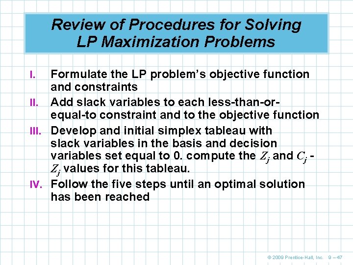
Review of Procedures for Solving LP Maximization Problems Formulate the LP problem’s objective function and constraints II. Add slack variables to each less-than-orequal-to constraint and to the objective function III. Develop and initial simplex tableau with slack variables in the basis and decision variables set equal to 0. compute the Zj and Cj Zj values for this tableau. IV. Follow the five steps until an optimal solution has been reached I. © 2009 Prentice-Hall, Inc. 9 – 47

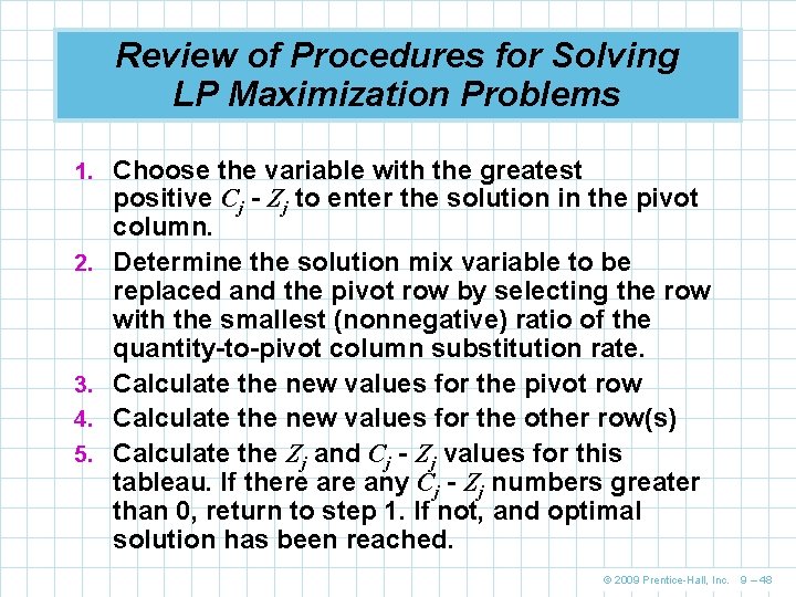
Review of Procedures for Solving LP Maximization Problems 1. Choose the variable with the greatest 2. 3. 4. 5. positive Cj - Zj to enter the solution in the pivot column. Determine the solution mix variable to be replaced and the pivot row by selecting the row with the smallest (nonnegative) ratio of the quantity-to-pivot column substitution rate. Calculate the new values for the pivot row Calculate the new values for the other row(s) Calculate the Zj and Cj - Zj values for this tableau. If there any Cj - Zj numbers greater than 0, return to step 1. If not, and optimal solution has been reached. © 2009 Prentice-Hall, Inc. 9 – 48

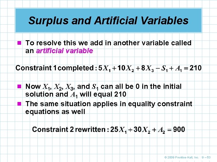
Surplus and Artificial Variables n Greater-than-or-equal-to (≥) constraints are just as common in real problems as less-than-or-equal-to (≤) constraints and equalities n To use the simplex method with these constraints, they must be converted to a special form similar to that made for the less-than-or-equal-to (≤) constraints n If they are not, the simplex technique is unable to set up an initial solution in the first tableau n Consider the following two constraints Constraint 1: 5 X 1 + 10 X 2 + 8 X 3 ≥ 210 Constraint 2: 25 X 1 + 30 X 2 = 900 © 2009 Prentice-Hall, Inc. 9 – 49

Surplus and Artificial Variables n Surplus variables n Greater-than-or-equal-to (≥) constraints require a different approach than the less-than-orequal-to (≤) constraints we have seen n They involve the subtraction of a surplus variable rather than the addition of a slack variable n The surplus variable tells us how much the solution exceeds the constraint amount n This is sometimes called negative slack © 2009 Prentice-Hall, Inc. 9 – 50

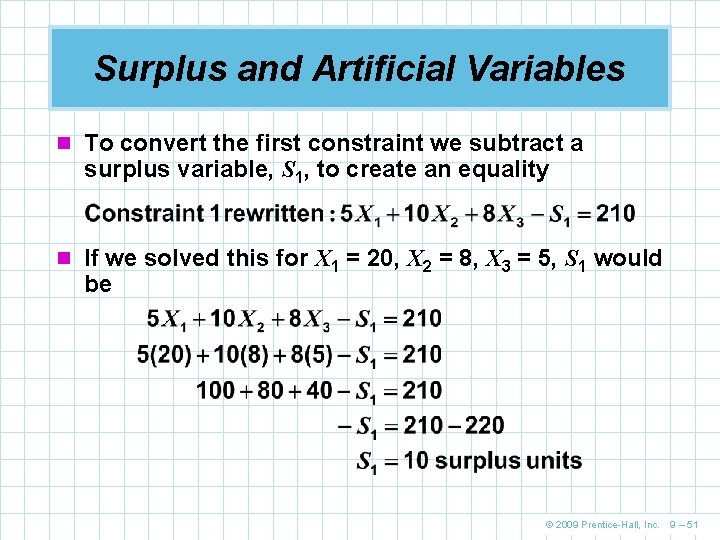
Surplus and Artificial Variables n To convert the first constraint we subtract a surplus variable, S 1, to create an equality n If we solved this for X 1 = 20, X 2 = 8, X 3 = 5, S 1 would be © 2009 Prentice-Hall, Inc. 9 – 51

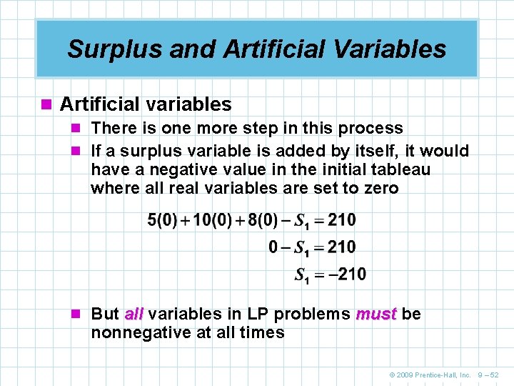
Surplus and Artificial Variables n Artificial variables n There is one more step in this process n If a surplus variable is added by itself, it would have a negative value in the initial tableau where all real variables are set to zero n But all variables in LP problems must be nonnegative at all times © 2009 Prentice-Hall, Inc. 9 – 52

Surplus and Artificial Variables n To resolve this we add in another variable called an artificial variable n Now X 1, X 2, X 3, and S 1 can all be 0 in the initial solution and A 1 will equal 210 n The same situation applies in equality constraint equations as well © 2009 Prentice-Hall, Inc. 9 – 53

Surplus and Artificial Variables n Artificial variables are inserted into equality n n constraints so we can easily develop an initial feasible solution When a problem has many constraint equations with many variables, it is not possible to “eyeball” an initial solution Using artificial variables allows us to use the automatic initial solution of setting all the other variables to 0 Unlike slack or surplus variables, artificial variables have no meaning in the problem formulation They are strictly a computational tool, they will be gone in the final solution © 2009 Prentice-Hall, Inc. 9 – 54

Surplus and Artificial Variables n Surplus and artificial variables in the objective function n Both types of variables must be included in the objective function n Surplus variables, like slack variables, carry a $0 cost coefficient n Since artificial variables must be forced out of the solution, we assign an arbitrarily high cost n By convention we use the coefficient M (or –M in maximization problems) which simply represents a very large number © 2009 Prentice-Hall, Inc. 9 – 55

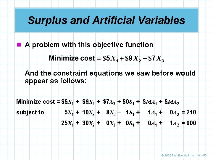
Surplus and Artificial Variables n A problem with this objective function And the constraint equations we saw before would appear as follows: Minimize cost = $5 X 1 + $9 X 2 + $7 X 3 + $0 S 1 + $MA 2 subject to 5 X 1 + 10 X 2 + 8 X 3 – 1 S 1 + 1 A 1 + 0 A 2 = 210 25 X 1 + 30 X 2 + 0 X 3 + 0 S 1 + 0 A 1 + 1 A 2 = 900 © 2009 Prentice-Hall, Inc. 9 – 56

Solving Minimization Problems n Once the necessary equations are developed for a minimization problem, we can use the simplex method to solve for an optimal solution © 2009 Prentice-Hall, Inc. 9 – 57

The Muddy River Chemical Corporation Example n The Muddy River Chemical Corporation must produce exactly 1, 000 pounds of a special mixture of phosphate and potassium for a customer n Phosphate costs $5 per pound and potassium $6 per pound n No more than 300 pounds of phosphate can be used and at least 150 pounds of potassium must be used n The company wants to find the least-cost blend of the two ingredients © 2009 Prentice-Hall, Inc. 9 – 58

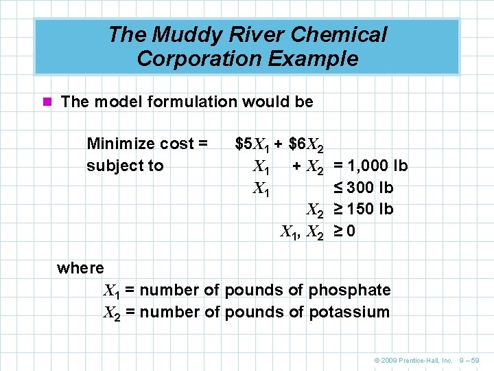
The Muddy River Chemical Corporation Example n The model formulation would be Minimize cost = subject to $5 X 1 + $6 X 2 X 1 + X 2 X 1, X 2 = 1, 000 lb ≤ 300 lb ≥ 150 lb ≥ 0 where X 1 = number of pounds of phosphate X 2 = number of pounds of potassium © 2009 Prentice-Hall, Inc. 9 – 59

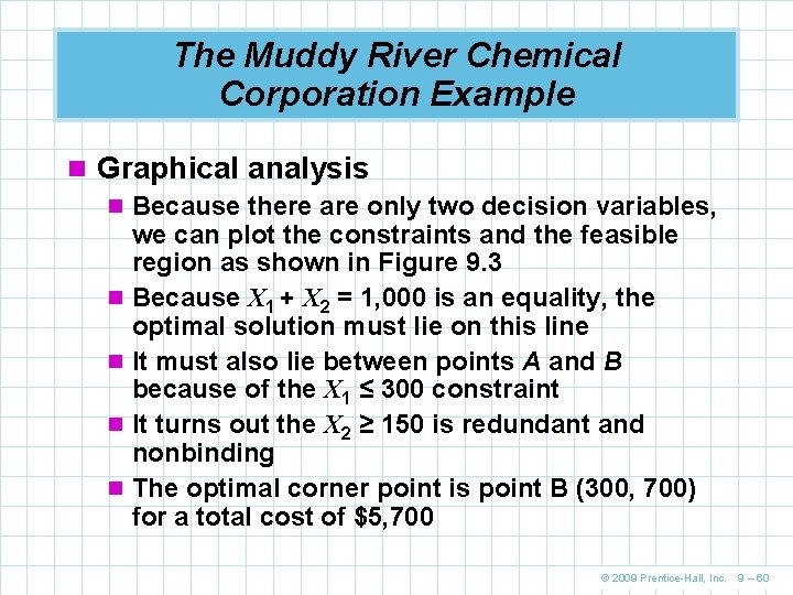
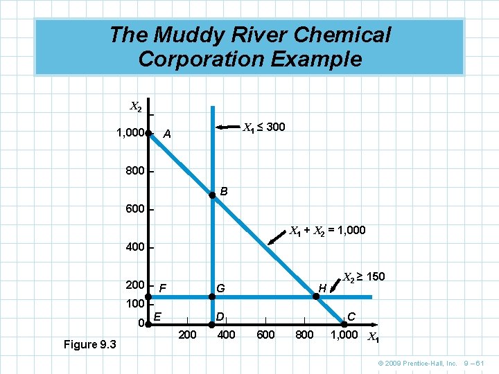
The Muddy River Chemical Corporation Example n Graphical analysis n Because there are only two decision variables, we can plot the constraints and the feasible region as shown in Figure 9. 3 n Because X 1 + X 2 = 1, 000 is an equality, the optimal solution must lie on this line n It must also lie between points A and B because of the X 1 ≤ 300 constraint n It turns out the X 2 ≥ 150 is redundant and nonbinding n The optimal corner point is point B (300, 700) for a total cost of $5, 700 © 2009 Prentice-Hall, Inc. 9 – 60

The Muddy River Chemical Corporation Example X 2 – X 1 ≤ 300 1, 000 – A 800 – B 600 – X 1 + X 2 = 1, 000 400 – 200 – F 100 – E 0 |– Figure 9. 3 G | 200 D| 400 H | | 600 800 X 2 ≥ 150 |C 1, 000 X 1 © 2009 Prentice-Hall, Inc. 9 – 61

The Muddy River Chemical Corporation Example n Rarely will problems be this simple n The simplex method can be used to solve much more complex problems n In this example, the simplex method will start at coroner point E, move to point F, then G and finally to point B which is the optimal solution © 2009 Prentice-Hall, Inc. 9 – 62

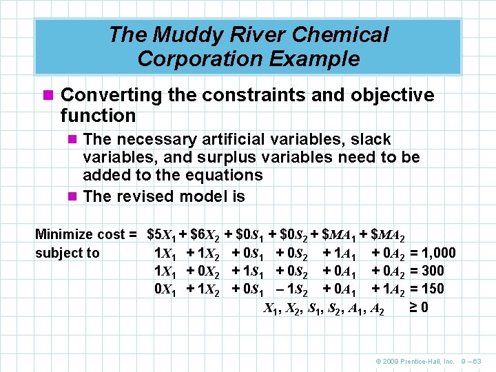
The Muddy River Chemical Corporation Example n Converting the constraints and objective function n The necessary artificial variables, slack variables, and surplus variables need to be added to the equations n The revised model is Minimize cost = $5 X 1 + $6 X 2 subject to 1 X 1 + 1 X 2 1 X 1 + 0 X 2 0 X 1 + 1 X 2 + $0 S 1 + 1 S 1 + 0 S 1 + $0 S 2 + $MA 1 + $MA 2 + 0 S 2 + 1 A 1 + 0 A 2 + 0 S 2 + 0 A 1 + 0 A 2 – 1 S 2 + 0 A 1 + 1 A 2 X 1 , X 2 , S 1 , S 2 , A 1 , A 2 = 1, 000 = 300 = 150 ≥ 0 © 2009 Prentice-Hall, Inc. 9 – 63

Rules of the Simplex Method for Minimization Problems n Minimization problems are quite similar to the n n n maximization problems tackled earlier The significant difference is the Cj - Zj row We will now choose the variable with the negative Cj - Zj that gives the largest improvement We select the variable that decreases costs the most In minimization problems, an optimal solution is reached when all the numbers in the Cj - Zj are 0 or positive All other steps in the simplex method remain the same © 2009 Prentice-Hall, Inc. 9 – 64

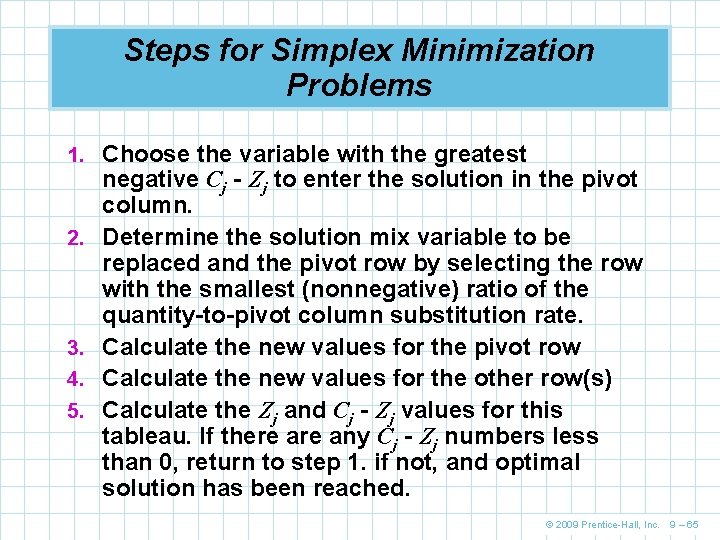
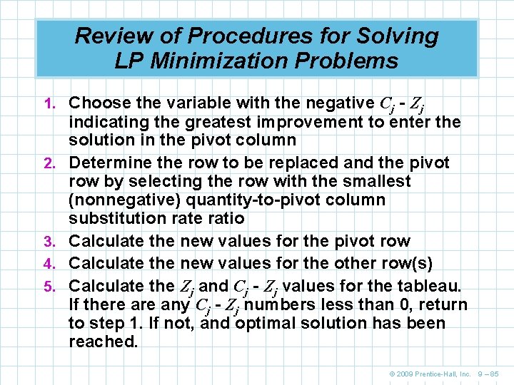
Steps for Simplex Minimization Problems 1. Choose the variable with the greatest 2. 3. 4. 5. negative Cj - Zj to enter the solution in the pivot column. Determine the solution mix variable to be replaced and the pivot row by selecting the row with the smallest (nonnegative) ratio of the quantity-to-pivot column substitution rate. Calculate the new values for the pivot row Calculate the new values for the other row(s) Calculate the Zj and Cj - Zj values for this tableau. If there any Cj - Zj numbers less than 0, return to step 1. if not, and optimal solution has been reached. © 2009 Prentice-Hall, Inc. 9 – 65

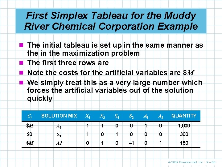
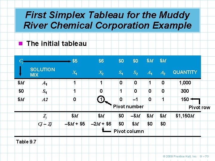
First Simplex Tableau for the Muddy River Chemical Corporation Example n The initial tableau is set up in the same manner as the in the maximization problem n The first three rows are n Note the costs for the artificial variables are $M n We simply treat this as a very large number which forces the artificial variables out of the solution quickly Cj SOLUTION MIX X 1 X 2 S 1 S 2 A 1 A 2 QUANTITY $M A 1 1 1 0 0 1, 000 $0 S 1 1 0 0 0 300 $M A 2 0 1 0 – 1 0 1 150 © 2009 Prentice-Hall, Inc. 9 – 66

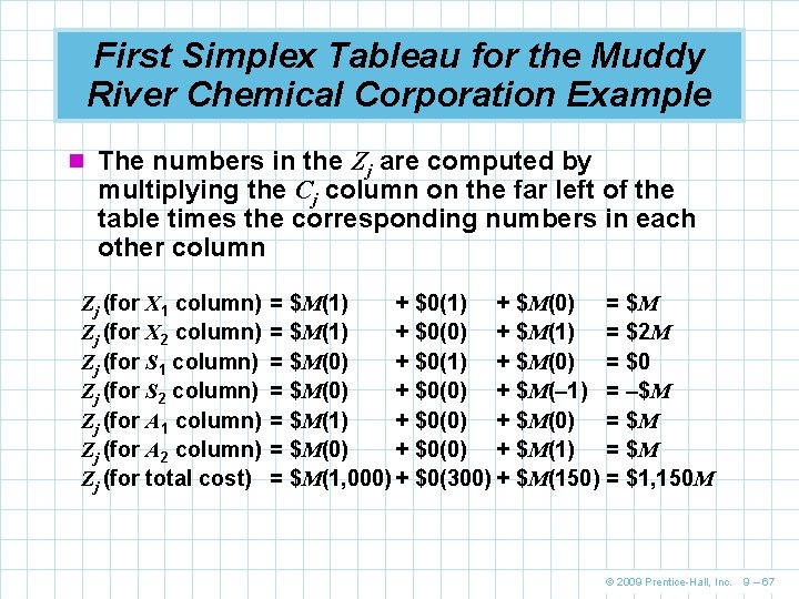
First Simplex Tableau for the Muddy River Chemical Corporation Example n The numbers in the Zj are computed by multiplying the Cj column on the far left of the table times the corresponding numbers in each other column Zj (for X 1 column) Zj (for X 2 column) Zj (for S 1 column) Zj (for S 2 column) Zj (for A 1 column) Zj (for A 2 column) Zj (for total cost) = $M(1) + $0(1) + $M(0) = $M(1) + $0(0) + $M(1) = $M(0) + $0(1) + $M(0) = $M(0) + $0(0) + $M(– 1) = $M(1) + $0(0) + $M(0) = $M(0) + $0(0) + $M(1) = $M(1, 000) + $0(300) + $M(150) = $M = $2 M = $0 = –$M = $1, 150 M © 2009 Prentice-Hall, Inc. 9 – 67

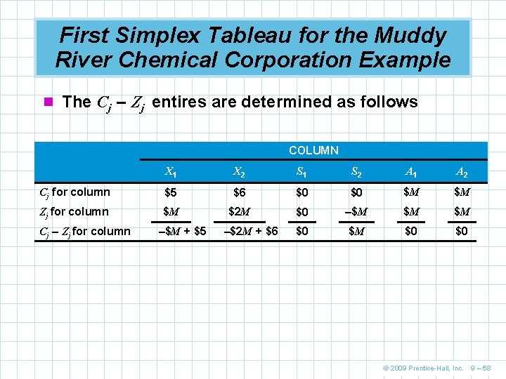
First Simplex Tableau for the Muddy River Chemical Corporation Example n The Cj – Zj entires are determined as follows COLUMN X 1 X 2 S 1 S 2 A 1 A 2 Cj for column $5 $6 $0 $0 $M $M Zj for column $M $2 M $0 –$M $M $M $0 $0 Cj – Zj for column –$M + $5 –$2 M + $6 © 2009 Prentice-Hall, Inc. 9 – 68

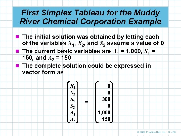
First Simplex Tableau for the Muddy River Chemical Corporation Example n The initial solution was obtained by letting each of the variables X 1, X 2, and S 2 assume a value of 0 n The current basic variables are A 1 = 1, 000, S 1 = 150, and A 2 = 150 n The complete solution could be expressed in vector form as X 1 X 2 S 1 S 2 A 1 A 2 = 0 0 300 0 1, 000 150 © 2009 Prentice-Hall, Inc. 9 – 69

First Simplex Tableau for the Muddy River Chemical Corporation Example n The initial tableau Cj SOLUTION MIX $5 $6 $0 $0 $M $M X 1 X 2 S 1 S 2 A 1 A 2 QUANTITY $M A 1 1 1 0 0 1, 000 $0 S 1 1 0 0 0 300 $M A 2 0 1 0 – 1 0 1 150 Pivot number Pivot row Zj $M $M $0 –$M $M $M Cj – Zj –$M + $5 – 2 M + $6 $0 $M $0 $0 $1, 150 M Pivot column Table 9. 7 © 2009 Prentice-Hall, Inc. 9 – 70

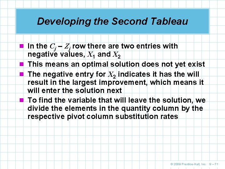
Developing the Second Tableau n In the Cj – Zj row there are two entries with negative values, X 1 and X 2 n This means an optimal solution does not yet exist n The negative entry for X 2 indicates it has the will result in the largest improvement, which means it will enter the solution next n To find the variable that will leave the solution, we divide the elements in the quantity column by the respective pivot column substitution rates © 2009 Prentice-Hall, Inc. 9 – 71

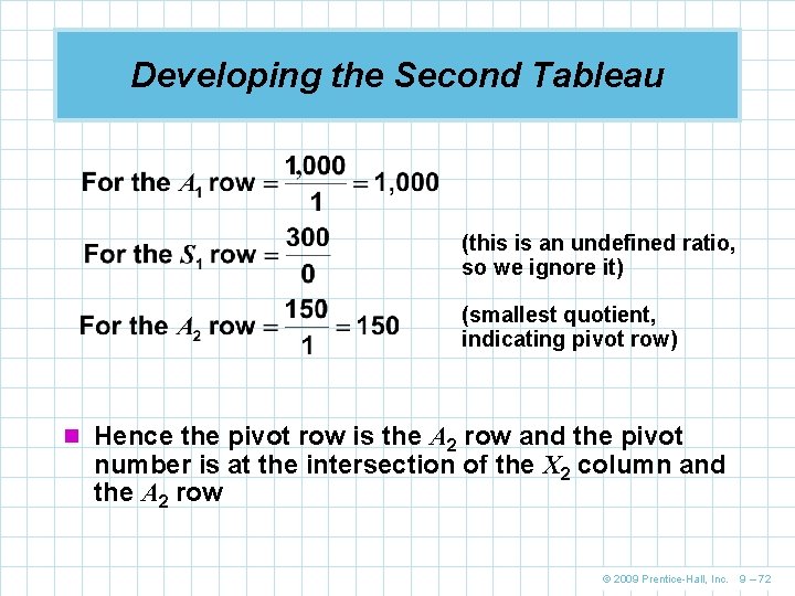
Developing the Second Tableau (this is an undefined ratio, so we ignore it) (smallest quotient, indicating pivot row) n Hence the pivot row is the A 2 row and the pivot number is at the intersection of the X 2 column and the A 2 row © 2009 Prentice-Hall, Inc. 9 – 72

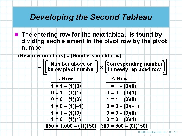
Developing the Second Tableau n The entering row for the next tableau is found by dividing each element in the pivot row by the pivot number (New row numbers) = (Numbers in old row) – Number above or below pivot number 1 0 0 1 1 – 1 850 Corresponding number in newly replaced row A 1 Row S 1 Row = 1 – (1)(0) 1 = 1 – (1)(1) 0 = 0 – (1)(0) 1 = 0 – (1)(– 1) 0 = 1 – (1)(0) 0 = 0 – (1)(1) 0 = 1, 000 – (1)(150) 300 = 1 – (0)(0) = 0 – (0)(1) = 1 – (0)(0) = 0 – (0)(– 1) = 0 – (0)(0) = 0 – (0)(1) = 300 – (0)(150) © 2009 Prentice-Hall, Inc. 9 – 73

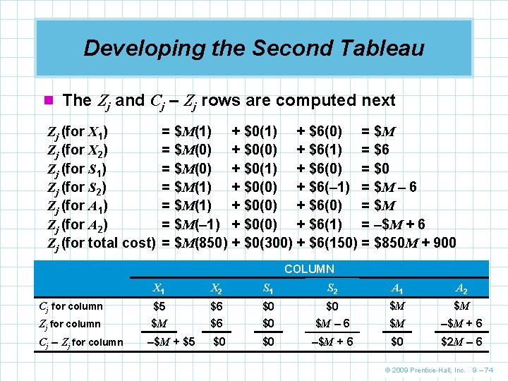
Developing the Second Tableau n The Zj and Cj – Zj rows are computed next Zj (for X 1) Zj (for X 2) Zj (for S 1) Zj (for S 2) Zj (for A 1) Zj (for A 2) Zj (for total cost) = $M(1) = $M(0) = $M(1) = $M(– 1) = $M(850) + $0(1) + $6(0) = $M + $0(0) + $6(1) = $6 + $0(1) + $6(0) = $0 + $0(0) + $6(– 1) = $M – 6 + $0(0) + $6(0) = $M + $0(0) + $6(1) = –$M + 6 + $0(300) + $6(150) = $850 M + 900 COLUMN X 1 X 2 S 1 S 2 A 1 A 2 Cj for column $5 $6 $0 $0 $M $M Zj for column $M $6 $0 $M – 6 $M –$M + 6 $0 $0 –$M + 6 $0 $2 M – 6 Cj – Zj for column –$M + $5 © 2009 Prentice-Hall, Inc. 9 – 74

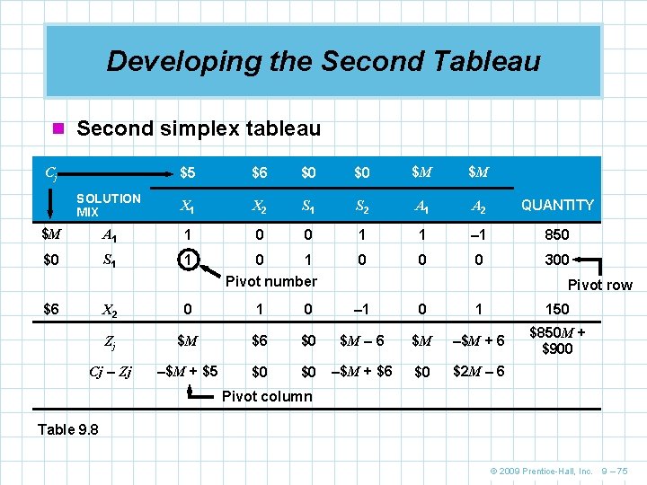
Developing the Second Tableau n Second simplex tableau $5 $6 $0 $0 $M $M SOLUTION MIX X 1 X 2 S 1 S 2 A 1 A 2 QUANTITY $M A 1 1 0 0 1 1 – 1 850 $0 S 1 1 0 0 0 300 Cj Pivot number $6 Pivot row X 2 0 1 0 – 1 0 1 150 Zj $M $6 $0 $M – 6 $M –$M + 6 $850 M + $900 Cj – Zj –$M + $5 $0 $0 –$M + $6 $0 $2 M – 6 Pivot column Table 9. 8 © 2009 Prentice-Hall, Inc. 9 – 75

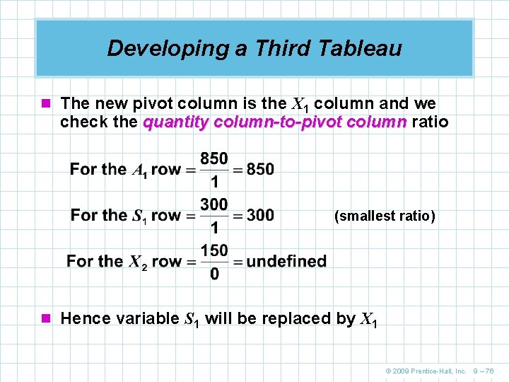
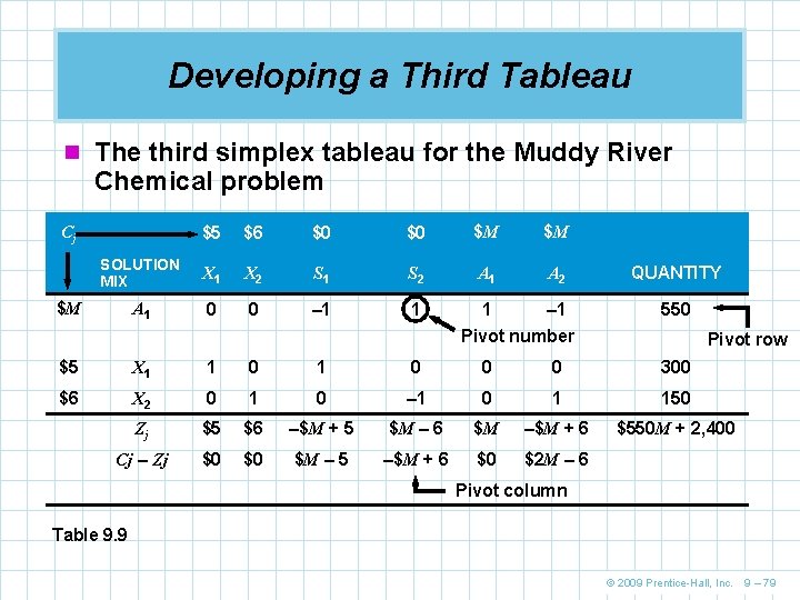
Developing a Third Tableau n The new pivot column is the X 1 column and we check the quantity column-to-pivot column ratio (smallest ratio) n Hence variable S 1 will be replaced by X 1 © 2009 Prentice-Hall, Inc. 9 – 76

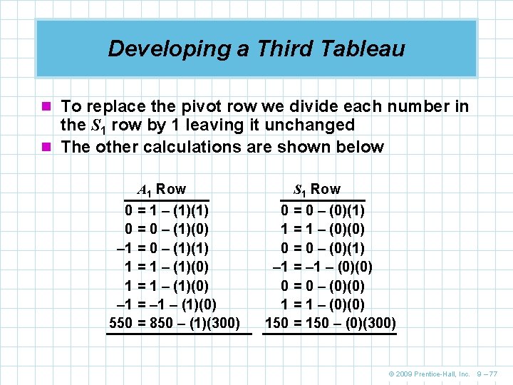
Developing a Third Tableau n To replace the pivot row we divide each number in the S 1 row by 1 leaving it unchanged n The other calculations are shown below A 1 Row 0 0 – 1 1 1 – 1 550 = 1 – (1)(1) = 0 – (1)(0) = 0 – (1)(1) = 1 – (1)(0) = – 1 – (1)(0) = 850 – (1)(300) S 1 Row 0 1 0 – 1 0 1 150 = 0 – (0)(1) = 1 – (0)(0) = 0 – (0)(1) = – 1 – (0)(0) = 0 – (0)(0) = 150 – (0)(300) © 2009 Prentice-Hall, Inc. 9 – 77

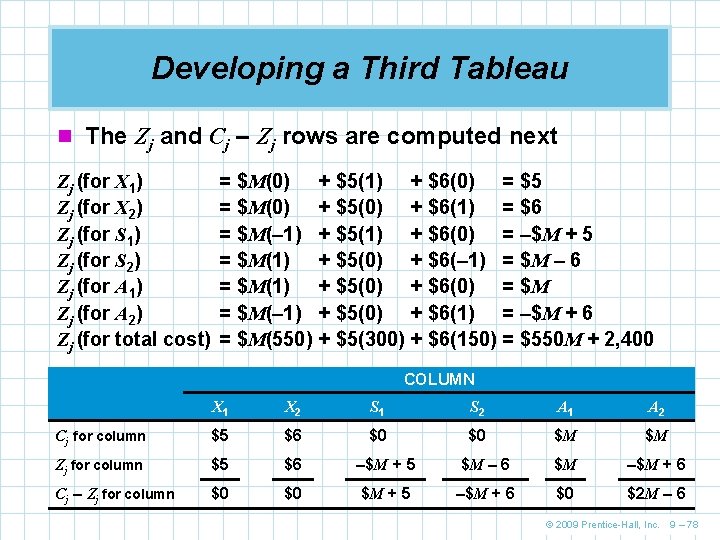
Developing a Third Tableau n The Zj and Cj – Zj rows are computed next Zj (for X 1) Zj (for X 2) Zj (for S 1) Zj (for S 2) Zj (for A 1) Zj (for A 2) Zj (for total cost) = $M(0) = $M(– 1) = $M(1) = $M(– 1) = $M(550) + $5(1) + $6(0) = $5 + $5(0) + $6(1) = $6 + $5(1) + $6(0) = –$M + 5 + $5(0) + $6(– 1) = $M – 6 + $5(0) + $6(0) = $M + $5(0) + $6(1) = –$M + 6 + $5(300) + $6(150) = $550 M + 2, 400 COLUMN X 1 X 2 S 1 S 2 A 1 A 2 Cj for column $5 $6 $0 $0 $M $M Zj for column $5 $6 –$M + 5 $M – 6 $M –$M + 6 Cj – Zj for column $0 $0 $M + 5 –$M + 6 $0 $2 M – 6 © 2009 Prentice-Hall, Inc. 9 – 78

Developing a Third Tableau n The third simplex tableau for the Muddy River Chemical problem $5 $6 $0 $0 $M $M SOLUTION MIX X 1 X 2 S 1 S 2 A 1 A 2 QUANTITY A 1 0 0 – 1 1 1 – 1 550 Cj $M Pivot number Pivot row $5 X 1 1 0 0 0 300 $6 X 2 0 1 0 – 1 0 1 150 Zj $5 $6 –$M + 5 $M – 6 $M –$M + 6 $550 M + 2, 400 Cj – Zj $0 $0 $M – 5 –$M + 6 $0 $2 M – 6 Pivot column Table 9. 9 © 2009 Prentice-Hall, Inc. 9 – 79

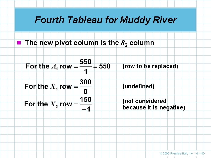
Fourth Tableau for Muddy River n The new pivot column is the S 2 column (row to be replaced) (undefined) (not considered because it is negative) © 2009 Prentice-Hall, Inc. 9 – 80

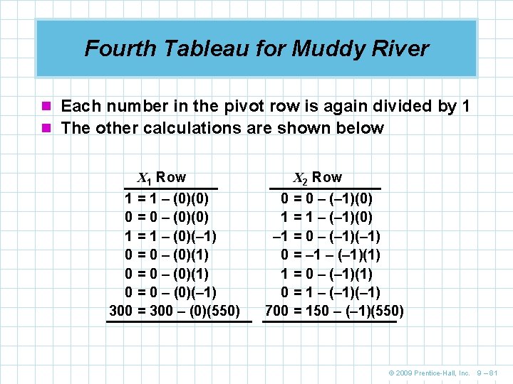
Fourth Tableau for Muddy River n Each number in the pivot row is again divided by 1 n The other calculations are shown below X 1 Row 1 0 0 0 300 = 1 – (0)(0) = 0 – (0)(0) = 1 – (0)(– 1) = 0 – (0)(1) = 0 – (0)(– 1) = 300 – (0)(550) X 2 Row 0 1 – 1 0 700 = 0 – (– 1)(0) = 1 – (– 1)(0) = 0 – (– 1) = – 1 – (– 1)(1) = 0 – (– 1)(1) = 1 – (– 1) = 150 – (– 1)(550) © 2009 Prentice-Hall, Inc. 9 – 81

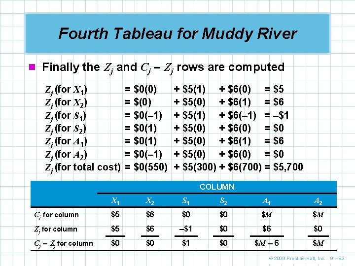
Fourth Tableau for Muddy River n Finally the Zj and Cj – Zj rows are computed Zj (for X 1) Zj (for X 2) Zj (for S 1) Zj (for S 2) Zj (for A 1) Zj (for A 2) Zj (for total cost) = $0(0) = $0(– 1) = $0(1) = $0(– 1) = $0(550) + $5(1) + $6(0) = $5 + $5(0) + $6(1) = $6 + $5(1) + $6(– 1) = –$1 + $5(0) + $6(0) = $0 + $5(0) + $6(1) = $6 + $5(0) + $6(0) = $0 + $5(300) + $6(700) = $5, 700 COLUMN X 1 X 2 S 1 S 2 A 1 A 2 Cj for column $5 $6 $0 $0 $M $M Zj for column $5 $6 –$1 $0 $6 $0 Cj – Zj for column $0 $0 $1 $0 $M – 6 $M © 2009 Prentice-Hall, Inc. 9 – 82

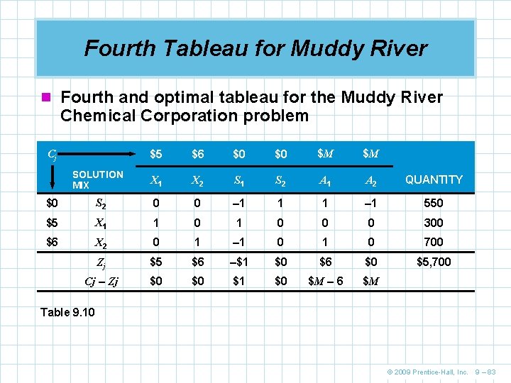
Fourth Tableau for Muddy River n Fourth and optimal tableau for the Muddy River Chemical Corporation problem Cj SOLUTION MIX $5 $6 $0 $0 $M $M X 1 X 2 S 1 S 2 A 1 A 2 QUANTITY $0 S 2 0 0 – 1 1 1 – 1 550 $5 X 1 1 0 0 0 300 $6 X 2 0 1 – 1 0 700 Zj $5 $6 –$1 $0 $6 $0 $5, 700 Cj – Zj $0 $0 $1 $0 $M – 6 $M Table 9. 10 © 2009 Prentice-Hall, Inc. 9 – 83

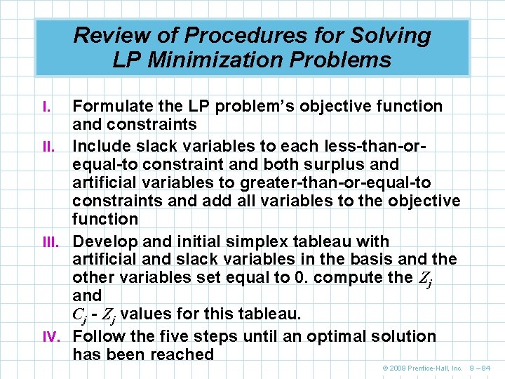
Review of Procedures for Solving LP Minimization Problems Formulate the LP problem’s objective function and constraints II. Include slack variables to each less-than-orequal-to constraint and both surplus and artificial variables to greater-than-or-equal-to constraints and add all variables to the objective function III. Develop and initial simplex tableau with artificial and slack variables in the basis and the other variables set equal to 0. compute the Zj and Cj - Zj values for this tableau. IV. Follow the five steps until an optimal solution has been reached I. © 2009 Prentice-Hall, Inc. 9 – 84

Review of Procedures for Solving LP Minimization Problems 1. Choose the variable with the negative Cj - Zj 2. 3. 4. 5. indicating the greatest improvement to enter the solution in the pivot column Determine the row to be replaced and the pivot row by selecting the row with the smallest (nonnegative) quantity-to-pivot column substitution rate ratio Calculate the new values for the pivot row Calculate the new values for the other row(s) Calculate the Zj and Cj - Zj values for the tableau. If there any Cj - Zj numbers less than 0, return to step 1. If not, and optimal solution has been reached. © 2009 Prentice-Hall, Inc. 9 – 85

Special Cases n We have seen how special cases arise when solving LP problems graphically n They also apply to the simplex method n You remember the four cases are n Infeasibility n Unbounded Solutions n Degeneracy n Multiple Optimal Solutions © 2009 Prentice-Hall, Inc. 9 – 86

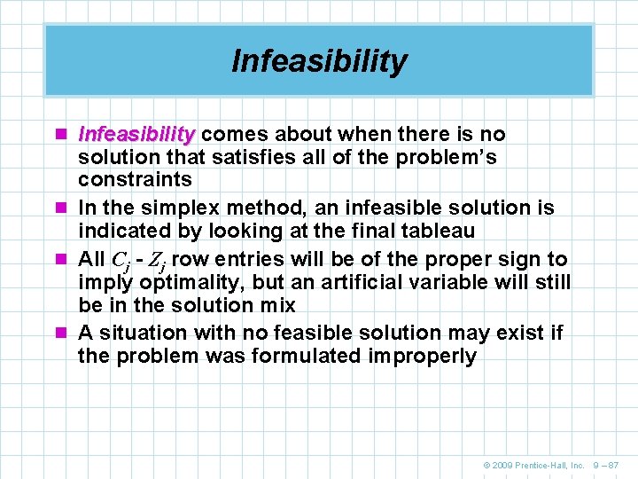
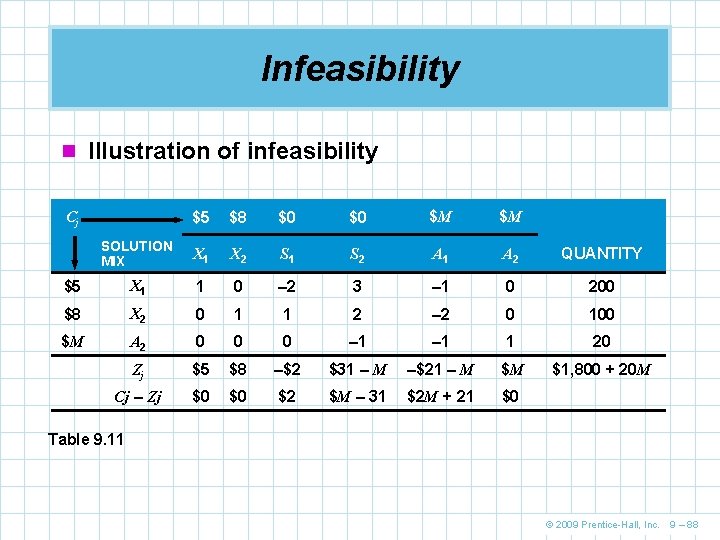
Infeasibility n Infeasibility comes about when there is no solution that satisfies all of the problem’s constraints n In the simplex method, an infeasible solution is indicated by looking at the final tableau n All Cj - Zj row entries will be of the proper sign to imply optimality, but an artificial variable will still be in the solution mix n A situation with no feasible solution may exist if the problem was formulated improperly © 2009 Prentice-Hall, Inc. 9 – 87

Infeasibility n Illustration of infeasibility $5 $8 $0 $0 $M $M SOLUTION MIX X 1 X 2 S 1 S 2 A 1 A 2 QUANTITY $5 X 1 1 0 – 2 3 – 1 0 200 $8 X 2 0 1 1 2 – 2 0 100 $M A 2 0 0 0 – 1 1 20 Zj $5 $8 –$2 $31 – M –$21 – M $M $1, 800 + 20 M Cj – Zj $0 $0 $2 $M – 31 $2 M + 21 $0 Cj Table 9. 11 © 2009 Prentice-Hall, Inc. 9 – 88

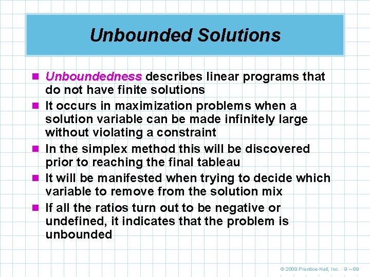
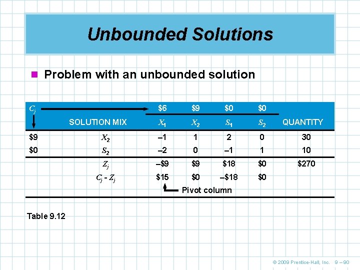
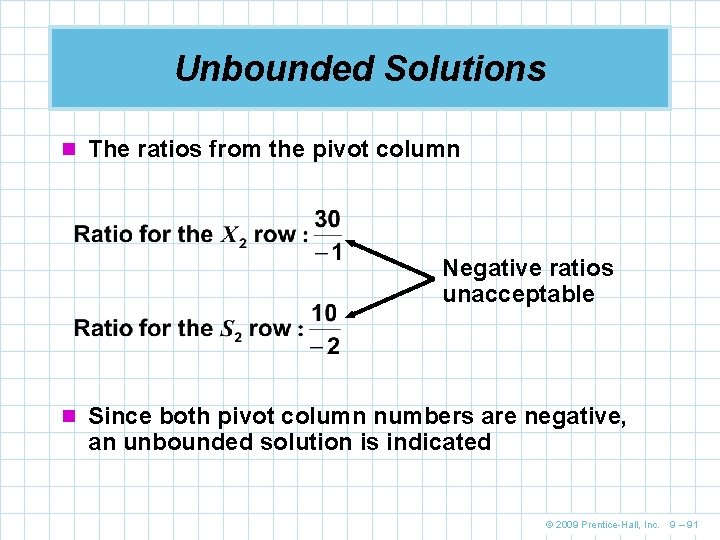
Unbounded Solutions n Unboundedness describes linear programs that n n do not have finite solutions It occurs in maximization problems when a solution variable can be made infinitely large without violating a constraint In the simplex method this will be discovered prior to reaching the final tableau It will be manifested when trying to decide which variable to remove from the solution mix If all the ratios turn out to be negative or undefined, it indicates that the problem is unbounded © 2009 Prentice-Hall, Inc. 9 – 89

Unbounded Solutions n Problem with an unbounded solution Cj SOLUTION MIX $6 $9 $0 $0 X 1 X 2 S 1 S 2 QUANTITY $9 X 2 – 1 1 2 0 30 $0 S 2 – 2 0 – 1 1 10 Zj –$9 $9 $18 $0 $270 Cj - Zj $15 $0 –$18 $0 Pivot column Table 9. 12 © 2009 Prentice-Hall, Inc. 9 – 90

Unbounded Solutions n The ratios from the pivot column Negative ratios unacceptable n Since both pivot column numbers are negative, an unbounded solution is indicated © 2009 Prentice-Hall, Inc. 9 – 91

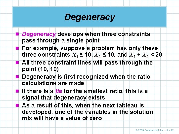
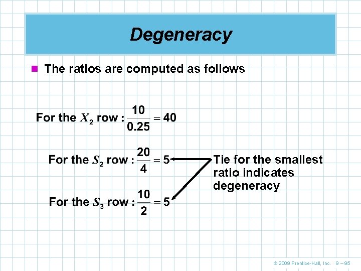
Degeneracy n Degeneracy develops when three constraints n n n pass through a single point For example, suppose a problem has only these three constraints X 1 ≤ 10, X 2 ≤ 10, and X 1 + X 2 < 20 All three constraint lines will pass through the point (10, 10) Degeneracy is first recognized when the ratio calculations are made If there is a tie for the smallest ratio, this is a signal that degeneracy exists As a result of this, when the next tableau is developed, one of the variables in the solution mix will have a value of zero © 2009 Prentice-Hall, Inc. 9 – 92

Degeneracy n Degeneracy could lead to a situation known as cycling in which the simplex algorithm alternates back and forth between the same nonoptimal solutions n One simple way of dealing with the issue is to select either row in question arbitrarily n If unlucky and cycling does occur, simply go back and select the other row © 2009 Prentice-Hall, Inc. 9 – 93

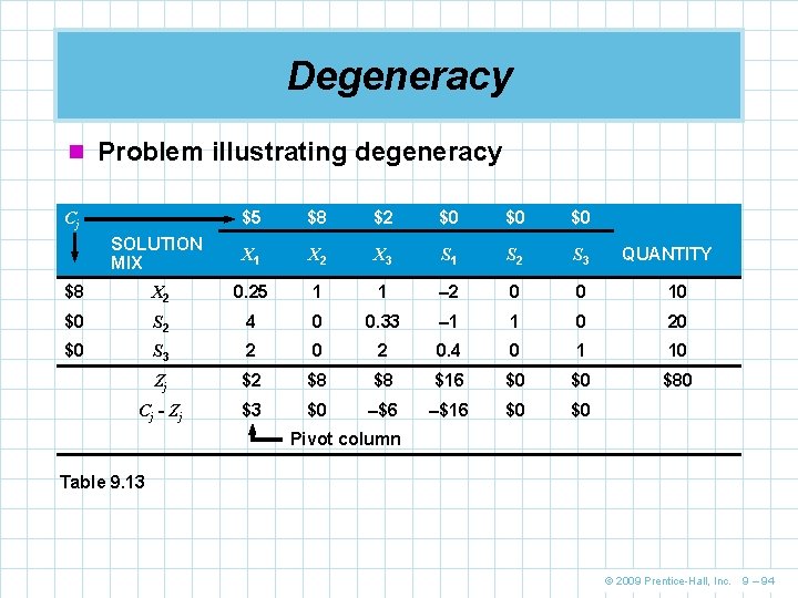
Degeneracy n Problem illustrating degeneracy $5 $8 $2 $0 $0 $0 SOLUTION MIX X 1 X 2 X 3 S 1 S 2 S 3 $8 X 2 0. 25 1 1 – 2 0 0 10 $0 S 2 4 0 0. 33 – 1 1 0 20 $0 S 3 2 0. 4 0 1 10 Zj $2 $8 $8 $16 $0 $0 $80 Cj - Zj $3 $0 –$6 –$16 $0 $0 Cj QUANTITY Pivot column Table 9. 13 © 2009 Prentice-Hall, Inc. 9 – 94

Degeneracy n The ratios are computed as follows Tie for the smallest ratio indicates degeneracy © 2009 Prentice-Hall, Inc. 9 – 95

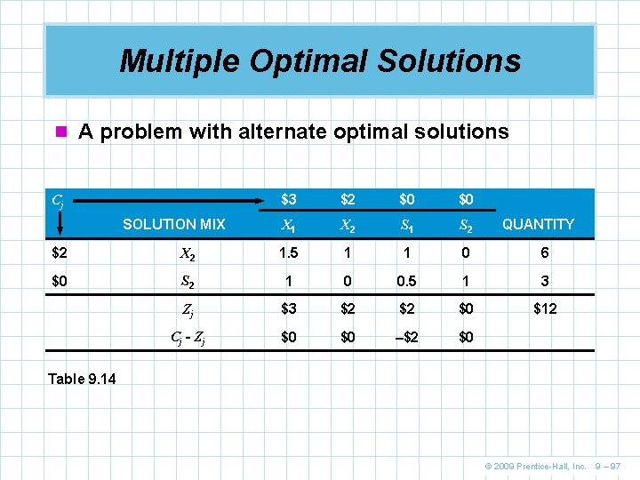
Multiple Optimal Solutions n In the simplex method, multiple, or alternate, optimal solutions can be spotted by looking at the final tableau n If the Cj – Zj value is equal to 0 for a variable that is not in the solution mix, more than one optimal solution exists © 2009 Prentice-Hall, Inc. 9 – 96

Multiple Optimal Solutions n A problem with alternate optimal solutions Cj SOLUTION MIX $3 $2 $0 $0 X 1 X 2 S 1 S 2 QUANTITY $2 X 2 1. 5 1 1 0 6 $0 S 2 1 0 0. 5 1 3 Zj $3 $2 $2 $0 $12 Cj - Zj $0 $0 –$2 $0 Table 9. 14 © 2009 Prentice-Hall, Inc. 9 – 97

Sensitivity Analysis with the Simplex Tableau n Sensitivity analysis shows how the optimal solution and the value of its objective function change given changes in various inputs to the problem n Computer programs handling LP problems of all sizes provide sensitivity analysis as an important output feature n Those programs use the information provided in the final simplex tableau to compute ranges for the objective function coefficients and ranges for the RHS values n They also provide “shadow prices, ” a concept we will introduce in this section © 2009 Prentice-Hall, Inc. 9 – 98

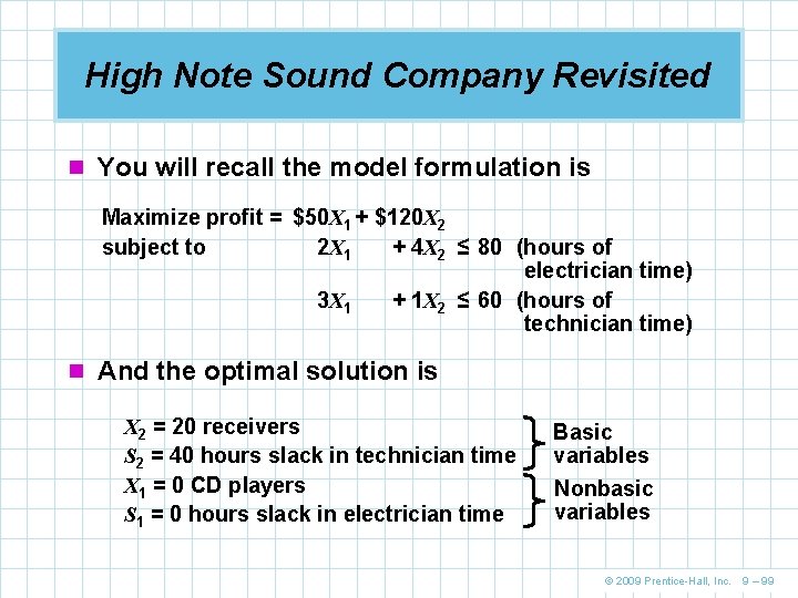
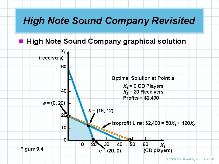
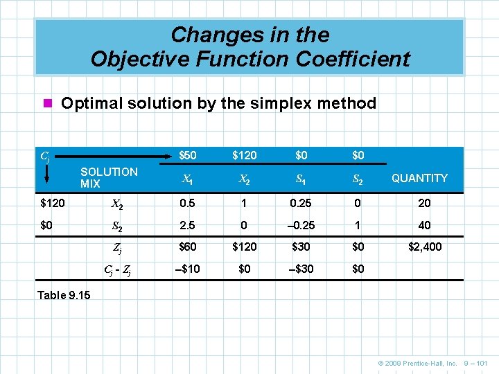
High Note Sound Company Revisited n You will recall the model formulation is Maximize profit = $50 X 1 + $120 X 2 subject to 2 X 1 + 4 X 2 ≤ 80 (hours of electrician time) 3 X 1 + 1 X 2 ≤ 60 (hours of technician time) n And the optimal solution is X 2 = 20 receivers S 2 = 40 hours slack in technician time X 1 = 0 CD players S 1 = 0 hours slack in electrician time Basic variables Nonbasic variables © 2009 Prentice-Hall, Inc. 9 – 99

High Note Sound Company Revisited n High Note Sound Company graphical solution X 2 (receivers) 60 – Optimal Solution at Point a – X 1 = 0 CD Players X 2 = 20 Receivers Profits = $2, 400 40 – a = (0, 20) – b = (16, 12) 20 – Isoprofit Line: $2, 400 = 50 X 1 + 120 X 2 10 – 0– Figure 9. 4 | | 10 20 | | 30 40 c = (20, 0) | 50 | 60 X 1 (CD players) © 2009 Prentice-Hall, Inc. 9 – 100

Changes in the Objective Function Coefficient n Optimal solution by the simplex method Cj SOLUTION MIX $50 $120 $0 $0 X 1 X 2 S 1 S 2 QUANTITY $120 X 2 0. 5 1 0. 25 0 20 $0 S 2 2. 5 0 – 0. 25 1 40 Zj $60 $120 $30 $0 $2, 400 Cj - Zj –$10 $0 –$30 $0 Table 9. 15 © 2009 Prentice-Hall, Inc. 9 – 101

Changes in the Objective Function Coefficient n Nonbasic objective function coefficient n The goal is to find out how sensitive the problem’s optimal solution is to changes in the contribution rates of variables not currently in the basis n How much would the objective function coefficients have to change before X 1 or S 1 would enter the solution mix and replace one of the basic variables? n The answer lies in the Cj – Zj row of the final simplex tableau © 2009 Prentice-Hall, Inc. 9 – 102

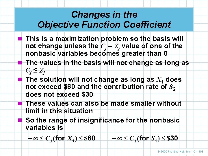
Changes in the Objective Function Coefficient n This is a maximization problem so the basis will n n not change unless the Cj – Zj value of one of the nonbasic variables becomes greater than 0 The values in the basis will not change as long as Cj ≤ Zj The solution will not change as long as X 1 does not exceed $60 and the contribution rate of S 2 does not exceed $30 These values can also be made smaller without limit in this situation So the range of insignificance for the nonbasic variables is © 2009 Prentice-Hall, Inc. 9 – 103

Changes in the Objective Function Coefficient n Basic objective function coefficient n Sensitivity analysis on objective function coefficients of variables in the basis or solution mix is slightly more complex n A change in the profit or cost of a basic variable can affect the Cj – Zj values for all nonbasic variables n That’s because the Cj value is in both the row and column n This then impacts the Cj – Zj row © 2009 Prentice-Hall, Inc. 9 – 104

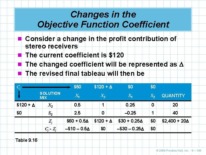
Changes in the Objective Function Coefficient n Consider a change in the profit contribution of stereo receivers n The current coefficient is $120 n The changed coefficient will be represented as n The revised final tableau will then be $50 $120 + $0 $0 SOLUTION MIX X 1 X 2 S 1 S 2 $120 + X 2 0. 5 1 0. 25 0 20 $0 S 2 2. 5 0 – 0. 25 1 40 Zj $60 + 0. 5 $120 + $30 + 0. 25 $0 $2, 400 + 20 Cj - Zj –$10 – 0. 5 $0 –$30 – 0. 25 $0 Cj QUANTITY Table 9. 16 © 2009 Prentice-Hall, Inc. 9 – 105

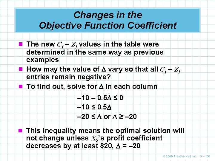
Changes in the Objective Function Coefficient n The new Cj – Zj values in the table were determined in the same way as previous examples n How may the value of vary so that all Cj – Zj entries remain negative? n To find out, solve for in each column – 10 – 0. 5 ≤ 0 – 10 ≤ 0. 5 – 20 ≤ or ≥ – 20 n This inequality means the optimal solution will not change unless X 2’s profit coefficient decreases by at least $20, = – 20 © 2009 Prentice-Hall, Inc. 9 – 106

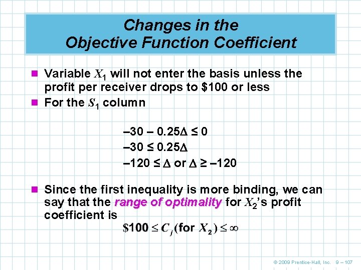
Changes in the Objective Function Coefficient n Variable X 1 will not enter the basis unless the profit per receiver drops to $100 or less n For the S 1 column – 30 – 0. 25 ≤ 0 – 30 ≤ 0. 25 – 120 ≤ or ≥ – 120 n Since the first inequality is more binding, we can say that the range of optimality for X 2’s profit coefficient is © 2009 Prentice-Hall, Inc. 9 – 107

Changes in the Objective Function Coefficient n In larger problems, we would use this procedure to test for the range of optimality of every real decision variable in the final solution mix n Using this procedure helps us avoid the timeconsuming process of reformulating and resolving the entire LP problem each time a small change occurs n Within the bounds, changes in profit coefficients will not force a change in the optimal solution n The value of the objective function will change, but this is a comparatively simple calculation © 2009 Prentice-Hall, Inc. 9 – 108

Changes in Resources or RHS Values n Making changes in the RHS values of constraints result in changes in the feasible region and often the optimal solution n Shadow prices n How much should a firm be willing to pay for one additional unit of a resource? n This is called the shadow price n Shadow pricing provides an important piece of economic information n This information is available in the final tableau © 2009 Prentice-Hall, Inc. 9 – 109

Changes in Resources or RHS Values n Final tableau for High Note Sound Cj SOLUTION MIX $50 $120 $0 $0 X 1 X 2 S 1 S 2 QUANTITY $120 X 2 0. 5 1 0. 25 0 20 $0 S 2 2. 5 0 – 0. 25 1 40 Zj $60 $120 $30 $0 $2, 400 Cj - Zj –$10 $0 –$30 $0 Objective function increases by $30 if 1 additional hour of electricians’ time is made available Table 9. 17 © 2009 Prentice-Hall, Inc. 9 – 110

Changes in Resources or RHS Values n An important property of the Cj – Zj row is that the n n negatives of the numbers in its slack variable (Si) columns provide us with shadow prices A shadow price is the change in value of the objective function from an increase of one unit of a scarce resource High Note Sound is considering hiring an extra electrician at $22 per hour In the final tableau we see S 1 (electricians’ time) is fully utilized and has a Cj – Zj value of –$30 They should hire the electrician as the firm will net $8 (= $30 – $22) © 2009 Prentice-Hall, Inc. 9 – 111

Changes in Resources or RHS Values n Should High Note Sound hire a part-time audio technician at $14 per hour? n In the final tableau we see S 2 (audio technician time) has slack capacity (40 hours) a Cj – Zj value of $0 n Thus there would be no benefit to hiring an additional audio technician © 2009 Prentice-Hall, Inc. 9 – 112

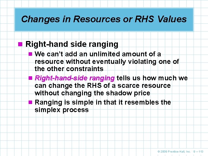
Changes in Resources or RHS Values n Right-hand side ranging n We can’t add an unlimited amount of a resource without eventually violating one of the other constraints n Right-hand-side ranging tells us how much we can change the RHS of a scarce resource without changing the shadow price n Ranging is simple in that it resembles the simplex process © 2009 Prentice-Hall, Inc. 9 – 113

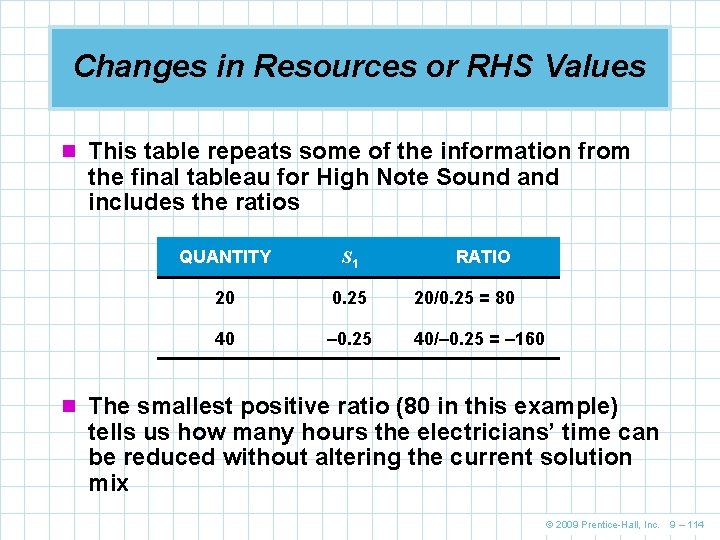
Changes in Resources or RHS Values n This table repeats some of the information from the final tableau for High Note Sound and includes the ratios QUANTITY S 1 RATIO 20 0. 25 20/0. 25 = 80 40 – 0. 25 40/– 0. 25 = – 160 n The smallest positive ratio (80 in this example) tells us how many hours the electricians’ time can be reduced without altering the current solution mix © 2009 Prentice-Hall, Inc. 9 – 114

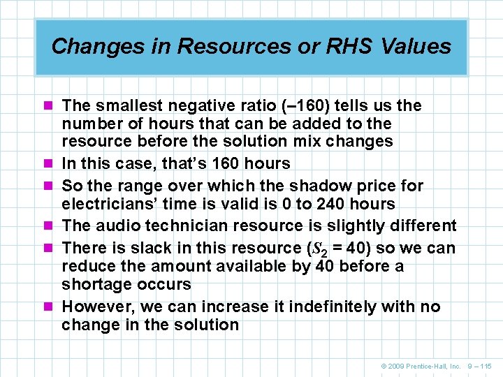
Changes in Resources or RHS Values n The smallest negative ratio (– 160) tells us the n n number of hours that can be added to the resource before the solution mix changes In this case, that’s 160 hours So the range over which the shadow price for electricians’ time is valid is 0 to 240 hours The audio technician resource is slightly different There is slack in this resource (S 2 = 40) so we can reduce the amount available by 40 before a shortage occurs However, we can increase it indefinitely with no change in the solution © 2009 Prentice-Hall, Inc. 9 – 115

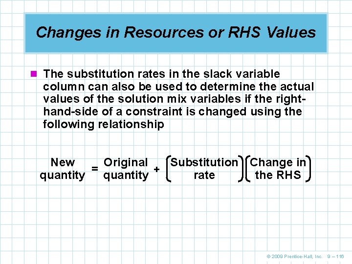
Changes in Resources or RHS Values n The substitution rates in the slack variable column can also be used to determine the actual values of the solution mix variables if the righthand-side of a constraint is changed using the following relationship New Original Substitution Change in = + quantity rate the RHS © 2009 Prentice-Hall, Inc. 9 – 116

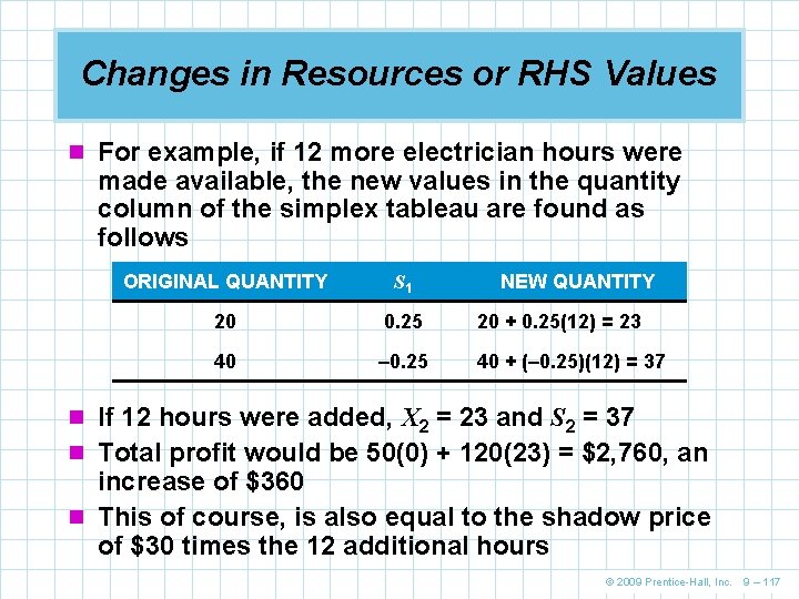
Changes in Resources or RHS Values n For example, if 12 more electrician hours were made available, the new values in the quantity column of the simplex tableau are found as follows ORIGINAL QUANTITY S 1 NEW QUANTITY 20 0. 25 20 + 0. 25(12) = 23 40 – 0. 25 40 + (– 0. 25)(12) = 37 n If 12 hours were added, X 2 = 23 and S 2 = 37 n Total profit would be 50(0) + 120(23) = $2, 760, an increase of $360 n This of course, is also equal to the shadow price of $30 times the 12 additional hours © 2009 Prentice-Hall, Inc. 9 – 117

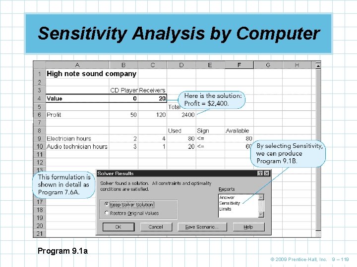
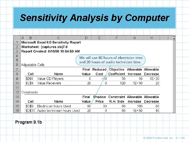
Sensitivity Analysis by Computer n Solver in Excel has the capability of producing sensitivity analysis that includes the shadow prices of resources n The following slides present the solution to the High Note Sound problem and the sensitivity report showing shadow prices and ranges © 2009 Prentice-Hall, Inc. 9 – 118

Sensitivity Analysis by Computer Program 9. 1 a © 2009 Prentice-Hall, Inc. 9 – 119

Sensitivity Analysis by Computer Program 9. 1 b © 2009 Prentice-Hall, Inc. 9 – 120

The Dual n Every LP problem has another LP problem n n associated with it called the dual The first way of stating a problem (what we have done so far) is called the primal The second way of stating it is called the dual The solutions to the primal and dual are equivalent, but they are derived through alternative procedures The dual contains economic information useful to managers and may be easier to formulate © 2009 Prentice-Hall, Inc. 9 – 121

The Dual n Generally, if the LP primal is a maximize profit problem with less-than-or-equal-to resource constraints, the dual will involve minimizing total opportunity cost subject to greater-than-or-equalto product profit constraints n Formulating a dual problem is not complex and once formulated, it is solved using the same procedure as a regular LP problem © 2009 Prentice-Hall, Inc. 9 – 122

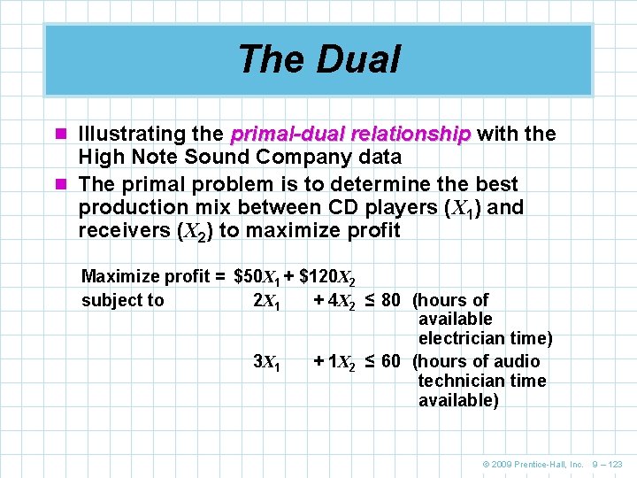
The Dual n Illustrating the primal-dual relationship with the High Note Sound Company data n The primal problem is to determine the best production mix between CD players (X 1) and receivers (X 2) to maximize profit Maximize profit = $50 X 1 + $120 X 2 subject to 2 X 1 + 4 X 2 ≤ 80 (hours of available electrician time) 3 X 1 + 1 X 2 ≤ 60 (hours of audio technician time available) © 2009 Prentice-Hall, Inc. 9 – 123

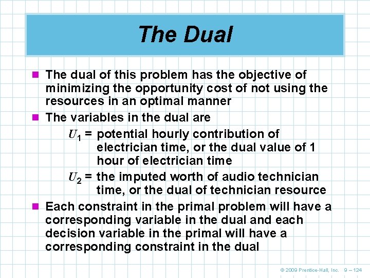
The Dual n The dual of this problem has the objective of minimizing the opportunity cost of not using the resources in an optimal manner n The variables in the dual are U 1 = potential hourly contribution of electrician time, or the dual value of 1 hour of electrician time U 2 = the imputed worth of audio technician time, or the dual of technician resource n Each constraint in the primal problem will have a corresponding variable in the dual and each decision variable in the primal will have a corresponding constraint in the dual © 2009 Prentice-Hall, Inc. 9 – 124

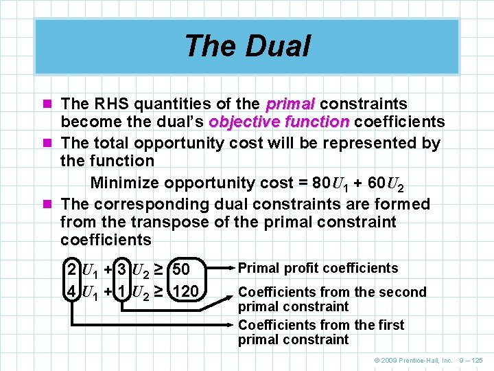
The Dual n The RHS quantities of the primal constraints become the dual’s objective function coefficients n The total opportunity cost will be represented by the function Minimize opportunity cost = 80 U 1 + 60 U 2 n The corresponding dual constraints are formed from the transpose of the primal constraint coefficients 2 U 1 + 3 U 2 ≥ 50 4 U 1 + 1 U 2 ≥ 120 Primal profit coefficients Coefficients from the second primal constraint Coefficients from the first primal constraint © 2009 Prentice-Hall, Inc. 9 – 125

The Dual n The first constraint says that the total imputed value or potential worth of the scarce resources needed to produce a CD player must be at least equal to the profit derived from the product n The second constraint makes an analogous statement for the stereo receiver product © 2009 Prentice-Hall, Inc. 9 – 126

Steps to Form the Dual n If the primal is a maximization problem in the n n standard form, the dual is a minimization, and vice versa The RHS values of the primal constraints become the dual’s objective coefficients The primal objective function coefficients become the RHS values of the dual constraints The transpose of the primal constraint coefficients become the dual constraint coefficients Constraint inequality signs are reversed © 2009 Prentice-Hall, Inc. 9 – 127

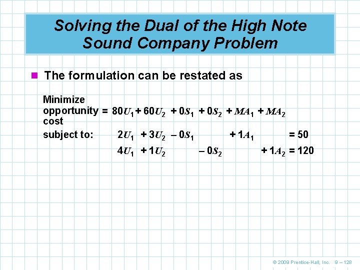
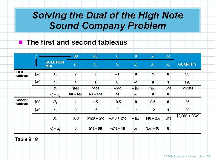
Solving the Dual of the High Note Sound Company Problem n The formulation can be restated as Minimize opportunity = 80 U 1 + 60 U 2 + 0 S 1 + 0 S 2 + MA 1 + MA 2 cost 2 U 1 + 3 U 2 – 0 S 1 + 1 A 1 = 50 subject to: 4 U 1 + 1 U 2 – 0 S 2 + 1 A 2 = 120 © 2009 Prentice-Hall, Inc. 9 – 128

Solving the Dual of the High Note Sound Company Problem n The first and second tableaus 80 60 0 0 M M SOLUTION MIX U 1 U 2 S 1 S 2 A 1 A 2 QUANTITY $M A 1 2 3 – 1 0 50 $M A 2 4 1 0 – 1 0 1 120 Zj $6 M $4 M –$M $M $M $170 M Cj – Z j 80 – 6 M 60 – 4 M M M 0 0 $80 U 1 1 1. 5 – 0. 5 0 25 $M A 2 0 – 5 2 – 1 – 2 1 20 Xj $80 $120 – 5 M –$40 + 2 M –$M $40 – 2 M $M Cj – Xj 0 5 M – 60 – 2 M + 40 M 3 M – 40 0 Cj First tableau Second tableau $2, 000 + 20 M Table 9. 18 © 2009 Prentice-Hall, Inc. 9 – 129

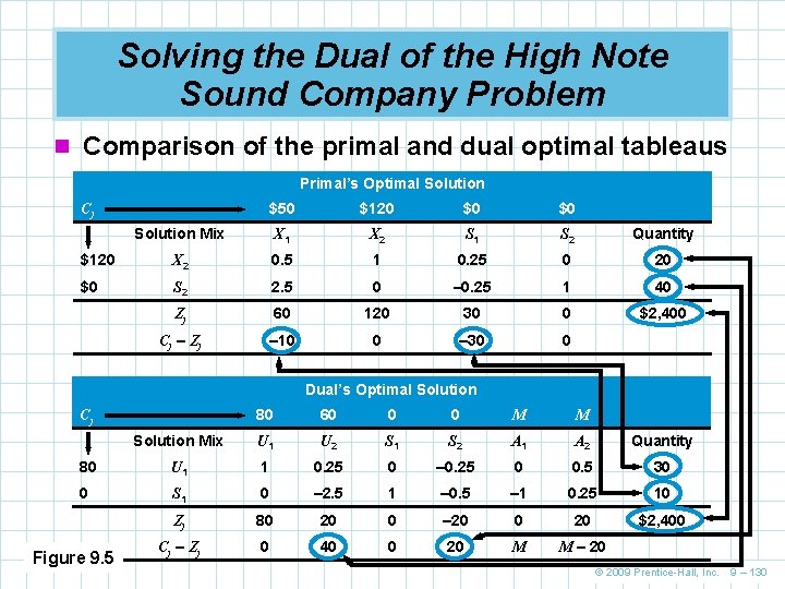
Solving the Dual of the High Note Sound Company Problem n Comparison of the primal and dual optimal tableaus Primal’s Optimal Solution $50 $120 $0 $0 Solution Mix X 1 X 2 S 1 S 2 Quantity $120 X 2 0. 5 1 0. 25 0 20 $0 S 2 2. 5 0 – 0. 25 1 40 Zj 60 120 30 0 $2, 400 Cj – Zj – 10 0 – 30 0 Cj Dual’s Optimal Solution 80 60 0 0 M M Solution Mix U 1 U 2 S 1 S 2 A 1 A 2 Quantity 80 U 1 1 0. 25 0 – 0. 25 0 0. 5 30 0 S 1 0 – 2. 5 1 – 0. 5 – 1 0. 25 10 Zj 80 20 0 – 20 0 20 $2, 400 Cj – Zj 0 40 0 20 M M – 20 Cj Figure 9. 5 © 2009 Prentice-Hall, Inc. 9 – 130

Solving the Dual of the High Note Sound Company Problem n In the final simplex tableau of a primal problem, the absolute values of the numbers in the Cj – Zj row under the slack variables represent the solutions to the dual problem n They are shadow prices in the primal solution and marginal profits in the dual n The absolute value of the numbers of the Cj – Zj values of the slack variables represent the optimal values of the primal X 1 and X 2 variables n The maximum opportunity cost derived in the dual must always equal the maximum profit derived in the primal © 2009 Prentice-Hall, Inc. 9 – 131

Karmakar’s Algorithm n In 1984, Narendra Karmakar developed a new n n method of solving linear programming problems called the Karmakar algorithm The simplex method follows a path of points on the outside edge of feasible space Karmakar’s algorithm works by following a path a points inside the feasible space It is much more efficient than the simplex method requiring less computer time to solve problems It can also handle extremely large problems allowing organizations to solve previously unsolvable problems © 2009 Prentice-Hall, Inc. 9 – 132