Mathematical Models in Neural and Neuroendocrine Systems Richard

Mathematical Models in Neural and Neuroendocrine Systems Richard Bertram Department of Mathematics and Programs in Neuroscience and Molecular Biophysics Florida State University

What’s the Point? n n n Integrate biological data Writing down equations often identifies holes in biological knowledge Use of math models helps to determine if data are logically consistent Making testable predictions Models force simplification, which can help in the identification of essential elements

How Much Detail Should Go Into a Model? Some reasons that simpler is better: n More detail means more undetermined parameters n More equations decrease our ability to comprehend the behavior of the model n Added detail can be misleading. It can give the false impression that all the components are necessary for the behavior

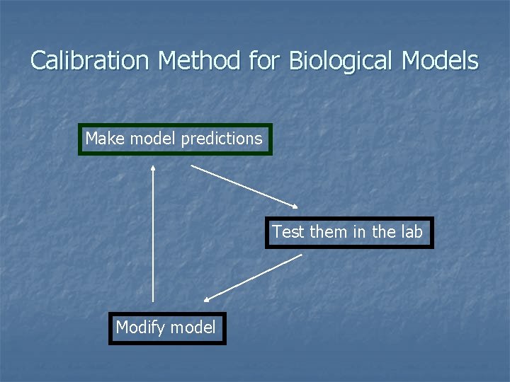
How Should One Calibrate a Biological Model? In engineering, one does experiments to determine the values of each parameter

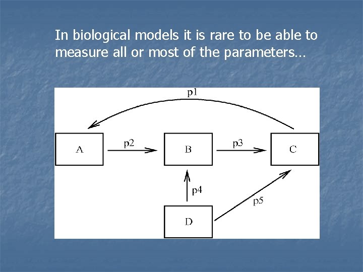
In biological models it is rare to be able to measure all or most of the parameters…

Calibration Method for Biological Models Make model predictions Test them in the lab Modify model

Single Cell Models

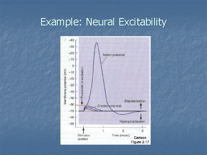
Example: Neural Excitability

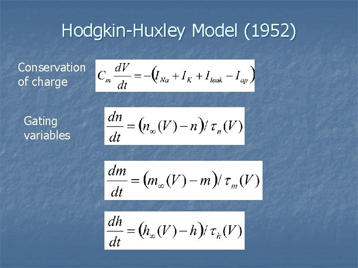
Hodgkin-Huxley Model (1952) Conservation of charge Gating variables

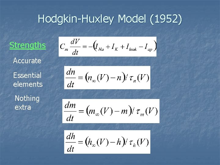
Hodgkin-Huxley Model (1952) Strengths Accurate Essential elements Nothing extra

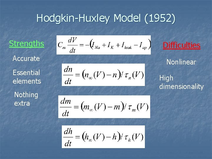
Hodgkin-Huxley Model (1952) Strengths Difficulties Accurate Nonlinear Essential elements Nothing extra High dimensionality

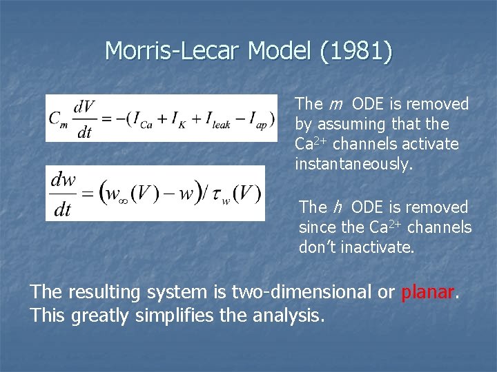
Morris-Lecar Model (1981) The m ODE is removed by assuming that the Ca 2+ channels activate instantaneously. The h ODE is removed since the Ca 2+ channels don’t inactivate. The resulting system is two-dimensional or planar. This greatly simplifies the analysis.

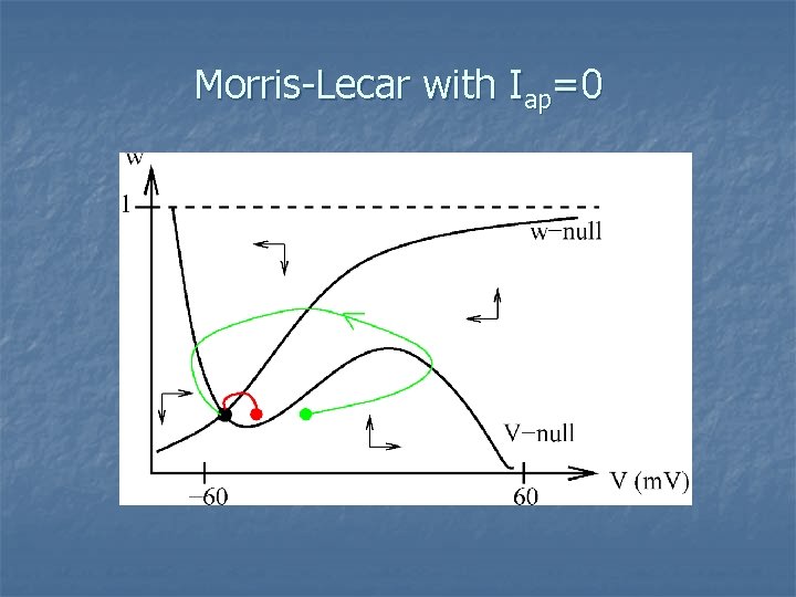
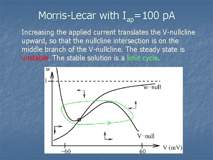
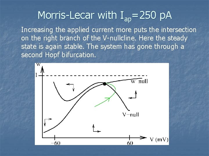
How do we analyze this? Phase plane: Study the dynamics in the Vw-plane rather than V or w versus time Nullclines: Determine the curves along which one of the time derivatives is 0 Steady states: At the intersections of the two nullclines both derivatives are 0, so the system is at rest Direction arrows: The nullclines divide up the plane, and the direction of flow in each region can be determined

Morris-Lecar with Iap=0

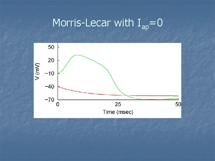
Morris-Lecar with Iap=0

Morris-Lecar with Iap=100 p. A Increasing the applied current translates the V-nullcline upward, so that the nullcline intersection is on the middle branch of the V-nullcline. The steady state is unstable. The stable solution is a limit cycle.

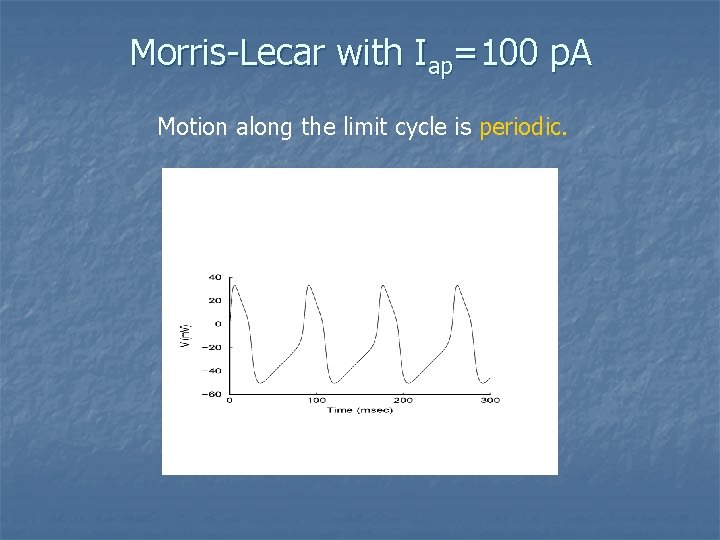
Morris-Lecar with Iap=100 p. A Motion along the limit cycle is periodic.

Hopf Bifurcation This transition from a stable steady state to a stable limit cycle through variation of a parameter is called a Hopf bifurcation. It is one way in which periodic motion can arise from a previously stationary system, or vice versa.

Morris-Lecar with Iap=250 p. A Increasing the applied current more puts the intersection on the right branch of the V-nullcline. Here the steady state is again stable. The system has gone through a second Hopf bifurcation.

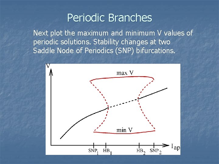
Bifurcation Diagrams These different behaviors and how they change with variation of a parameter can be summarized with a Bifurcation Diagram.

Stationary Branches For each value of the bifurcation parameter Iap plot the V value of the steady state solution. If stable make the curve solid; if unstable make the curve dashed. Stability changes at bifurcation points.

Periodic Branches Next plot the maximum and minimum V values of periodic solutions. Stability changes at two Saddle Node of Periodics (SNP) bifurcations.

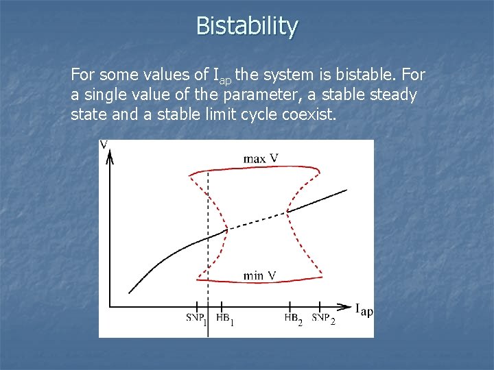
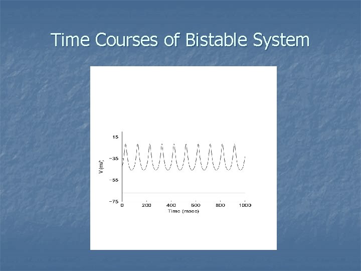
Bistability For some values of Iap the system is bistable. For a single value of the parameter, a stable steady state and a stable limit cycle coexist.

Bistability in the Phase Plane The unstable limit cycle (dashed) separates the basin of attraction of the steady state from that of the stable limit cycle. It is the separatrix.

Time Courses of Bistable System

Example 2: Calcium Dynamics Because Ca 2+ plays a large role in cells, modelers have used differential equations to describe the changes over time of the concentration of free Ca 2+ in the cytosol, endoplasmic reticulum, and in some cases in the mitochondria. We will derive equations for the free concentration in the cytosol and the ER, starting with the cytosol.

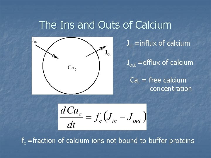
The Ins and Outs of Calcium Jin =influx of calcium Jout =efflux of calcium Cac = free calcium concentration fc =fraction of calcium ions not bound to buffer proteins

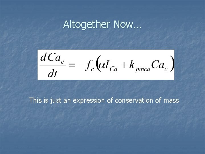
Calcium Flux Terms Influx of calcium is through ion channels, with current ICa: converts current to flux Efflux of calcium is through calcium pumps in the plasma membrane. We can approximate this pumping as proportional to the amount of free calcium in the cytosol: kpmca is the pump rate

Altogether Now… This is just an expression of conservation of mass

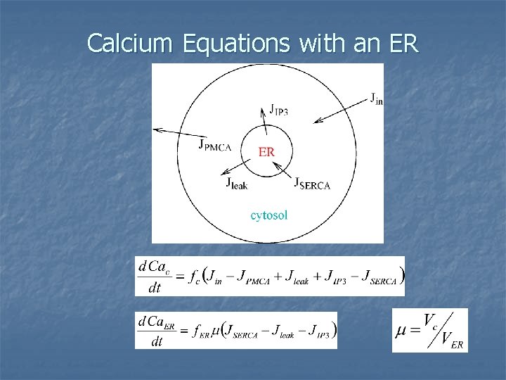
Calcium Equations with an ER

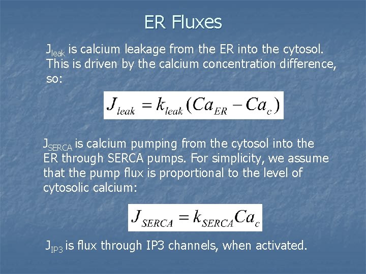
ER Fluxes Jleak is calcium leakage from the ER into the cytosol. This is driven by the calcium concentration difference, so: JSERCA is calcium pumping from the cytosol into the ER through SERCA pumps. For simplicity, we assume that the pump flux is proportional to the level of cytosolic calcium: JIP 3 is flux through IP 3 channels, when activated.

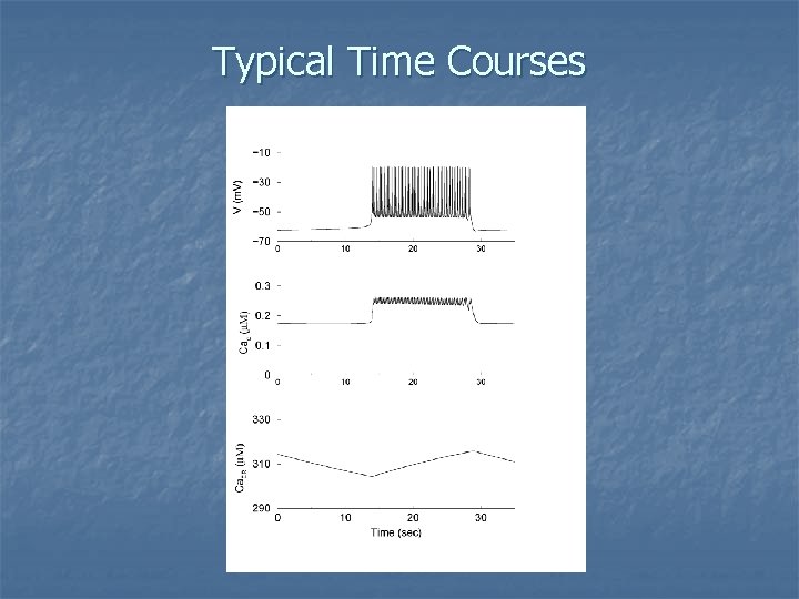
Typical Time Courses

Mean Field Models

What is Mean Field? These models are often used to describe the time dynamics of a large population of cells, where single-cell models would be inappropriate. With a mean field model a single variable would be used to describe, for example, the mean firing rate of a population of neurons. Usingle-cell models here would result in thousands of variables and equations.

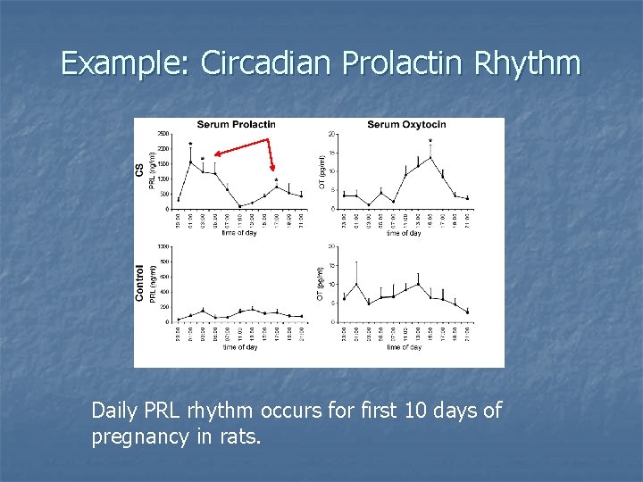
Example: Circadian Prolactin Rhythm Daily PRL rhythm occurs for first 10 days of pregnancy in rats.

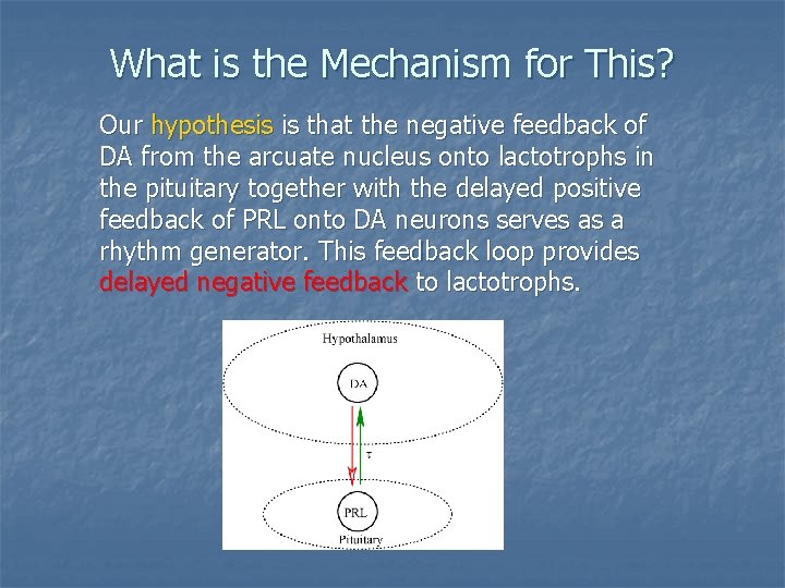
What is the Mechanism for This? Our hypothesis is that the negative feedback of DA from the arcuate nucleus onto lactotrophs in the pituitary together with the delayed positive feedback of PRL onto DA neurons serves as a rhythm generator. This feedback loop provides delayed negative feedback to lactotrophs.

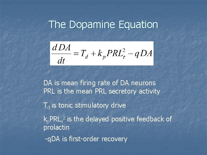
The Dopamine Equation DA is mean firing rate of DA neurons PRL is the mean PRL secretory activity Td is tonic stimulatory drive kp. PRL 2 is the delayed positive feedback of prolactin -q. DA is first-order recovery

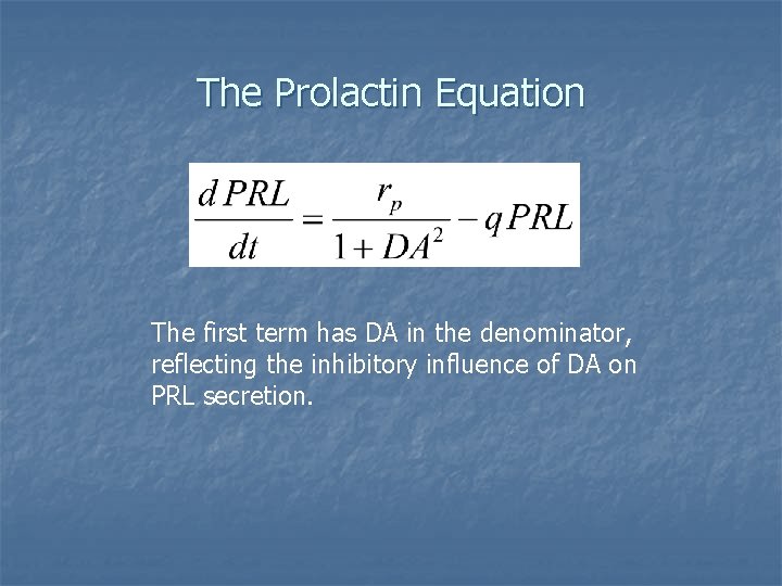
The Prolactin Equation The first term has DA in the denominator, reflecting the inhibitory influence of DA on PRL secretion.

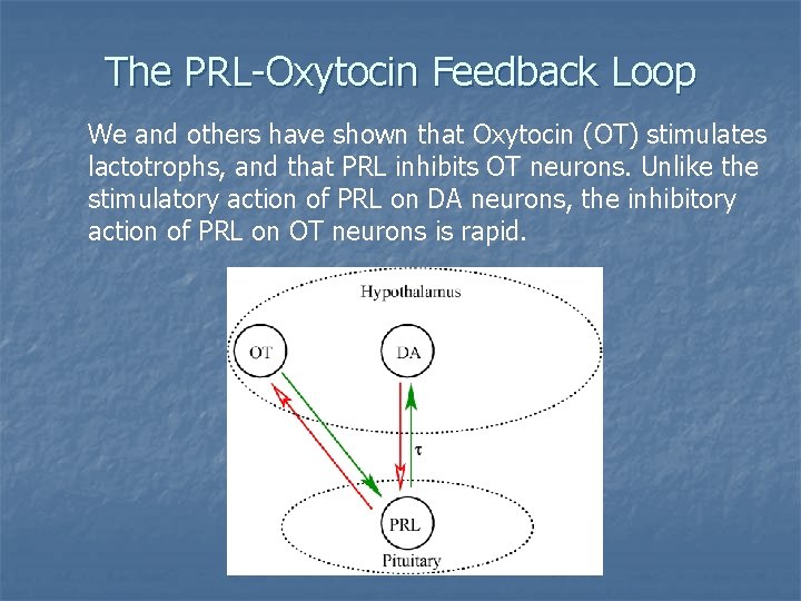
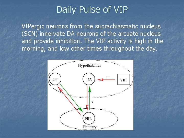
The PRL-Oxytocin Feedback Loop We and others have shown that Oxytocin (OT) stimulates lactotrophs, and that PRL inhibits OT neurons. Unlike the stimulatory action of PRL on DA neurons, the inhibitory action of PRL on OT neurons is rapid.

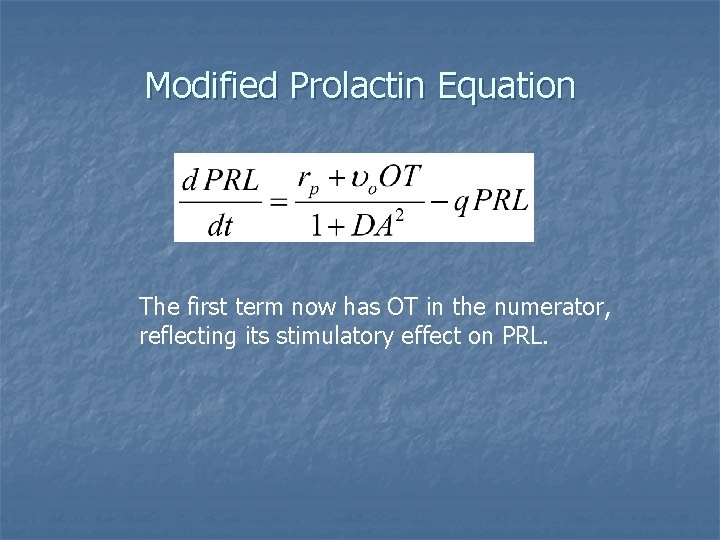
Modified Prolactin Equation The first term now has OT in the numerator, reflecting its stimulatory effect on PRL.

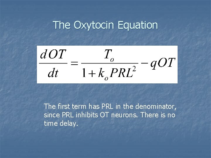
The Oxytocin Equation The first term has PRL in the denominator, since PRL inhibits OT neurons. There is no time delay.

Daily Pulse of VIPergic neurons from the suprachiasmatic nucleus (SCN) innervate DA neurons of the arcuate nucleus and provide inhibition. The VIP activity is high in the morning, and low other times throughout the day.

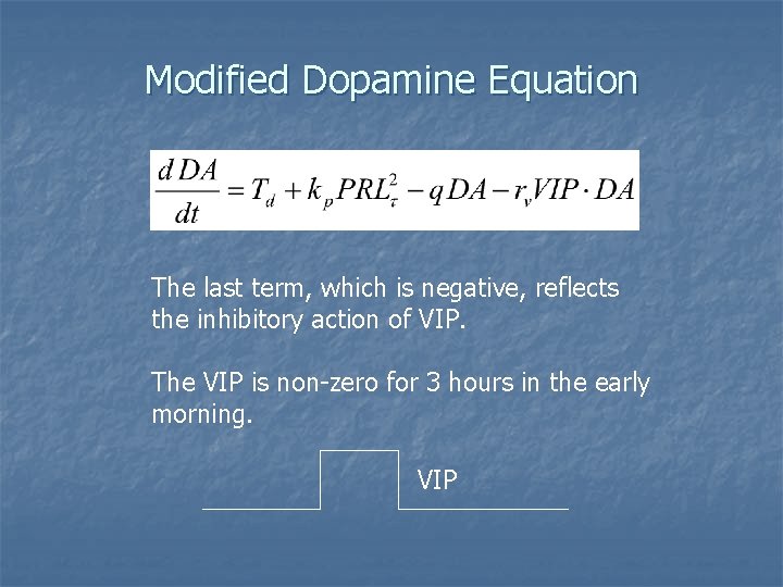
Modified Dopamine Equation The last term, which is negative, reflects the inhibitory action of VIP. The VIP is non-zero for 3 hours in the early morning. VIP

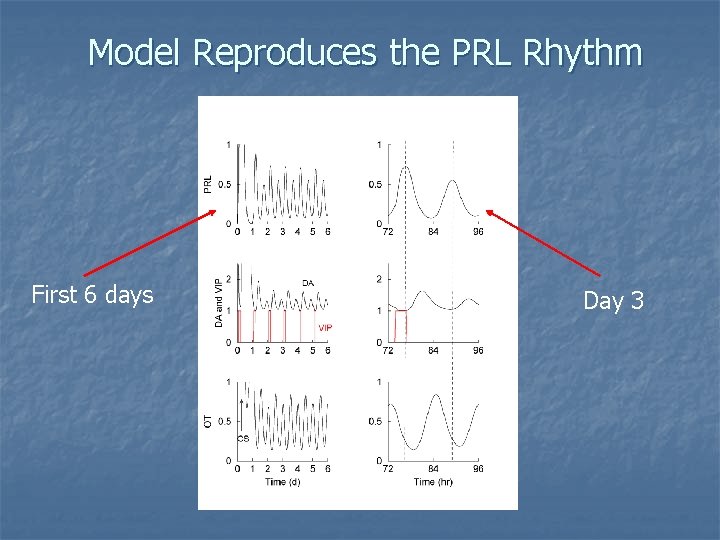
Model Reproduces the PRL Rhythm First 6 days Day 3

Uses of the Model We have used the PRL rhythm model to help in the design of experiments. Several predictions have been made and tested, and based on the results we have modified the model. It is a work in progress! Our goal with this mean field model is not to make quantitative predictions, but to make qualitative predictions. This is all that one can expect when thousands of cells are represented by a single variable!

Thanks to … Marc Freeman Marcel Egli The NIH and NSF for financial support