2 MATHEMATICAL MODELLING 2 Mathematical Modelling A mathematical

2. MATHEMATICAL MODELLING

2. Mathematical Modelling A mathematical model is an abstract model that uses mathematical language to describe the behaviour of a system. Mathematical models are used particularly in the natural sciences and engineering disciplines (such as physics, biology, and electrical engineering) but also in the social sciences

�Different systems contain different properties that are characterized using same mathematical expression. �Resistive property: Electrical resistance �Ohm’s Law: �Ohm's Law is the mathematical relationship among electric current, resistance, and voltage. The principle is named after the German scientist Georg Simon Ohm.

�Ohm's law states that the current through a conductor between two points is directly proportional to the potential difference across the two points. �I α V �V=IR ------- (1) �V is an “across” variable & viewed as a measure of effort. �I is a “through” variable & viewed as a measure of flow.

�V- across- effort variable - ψ �I- through- flow variable- ζ �Hence, V=IR, in generalized form it becomes: Ψ= ζR ---- (2)

Application of this generalized resistance to different kinds of systems. �Mechanical systems �Fluidic systems �Thermal systems �Chemical systems

Mechanical systems F α v, F = v Rm Rm =mechanical resistance. F= force applied v= velocity. F & v correspond to ψ & ζ v

2. Fluidic Ohm’s law – Poiseuille’s law. It states that “the volumetric flow of fluid Q, through a rigid tube is proportional to the pressure difference (∆P) across the two ends of the tube. ∆P = P 1 – P 2 ∆P α Q ∆P = Q Rf

3. Thermal Fourier’s Law “the flow of heat, Q, conducted through a given material is directly α The temperature difference that exists across the material. ∆θ α Q ∆θ= QRt

4. Chemical systems Fick’s Law “the flux Q of a given chemical species across a permeable membrane separating two fluids with different species concentration is α to the concentration difference, ∆φ. ∆φ= φ1 – φ2 ∆φ α Q ∆φ= Q Rc

Resistance property � 1. Mechanical systems F = v Rm � 2. Fluidic ∆P = Q Rf � 3. Thermal ∆θ= QRt � 4. Chemical systems ∆φ= Q Rc V=IR Ψ= ζR

Second generalized system property : Storage �In electrical systems, it takes the form of capacitance, defined as the amount of electrical charge (q) stored in the capacitor per unit voltage(V) that exists across the capacitor.

�q – accumulation of all electric charge delivered when current flow to the capacitor. � q= ʃo t I dt -----(1) C= q / v ------(2) V =Ψ The generalized formula : Ψ = 1/C ʃo t ζ I= ζ

1. Mechanical system �Storage property = compliance �X= FCm

2. Fluidic systems �Compliance determines the volume by which the balloon will expand or contract per unit change in applied pressure. ∆V (volume change) ∆P

3. Thermal systems �Thermal mass represents the amount of heat stored in a certain medium per unit difference in temperature that exists between the interior and exterior. �Heat stored, q= ∆θ Ct θ 2 �∆θ= θ 1 – θ 2 θ 1

4. Chemical systems �Here, the storage property is represented by the total volume of the fluid in which the chemical species exists. “ concentration”. �The storage element allows the accumulation of “static” or potential energy.

�The resistive & storage properties in an element represents the amount of energy store and dissipated. �In electric resistance, �Voltage * current = power.

� 1. Mechanical �Force * velocity = power � 2. Fluidic system �Pressure * flow rate = power

Inductance �“ the voltage required to produce a given rate of change of electric current” �V= L (d. I / dt) �Generalized system, � Ψ= L (dζ / dt)

�Mechanical systems : Newton’s second law of motion: �Force equals mass times acceleration. �Ψ - - force & ζ - - velocity. �Fluid = inertance α pressure differential applied. �Kinetic energy storage does not exist in thermal and chemical systems.

�Models with combinations of system elements The three basic model elements are linear.

Ψa ζ 1 Ψb E 1 a b E 2 ζ 3 E 3 0 �O= the reference level, electrical ground. �Ψa & Ψb= across variables at node a & b. �ζ 1, ζ 2 & ζ 3= through variables that pass through the elements E 1, E 2 & E 3

�Applying Kirchoff’s laws to the circuit: � 1. The algebraic sum of the “across-variable” values around any closed circuit must equal zero. Thus, in the loop a-b-o , �(Ψa – Ψb) + (Ψb-0)+(0 -Ψa)=0 � 2. The algebraic sum of all “through-variable” values into a given node must equal zero. �ζ 1 + (-ζ 2) + (-ζ 3)=0

Resultant system properties

Mechanical system �F = v Rm , resistances in series �F = v (Rm 1 + Rm 2 ), �X= FCm , capacitance in series �X= F[(Cm 1 + Cm 2 ) / (Cm 1 * Cm 2 )]

RESPIRATORY MECHANICS

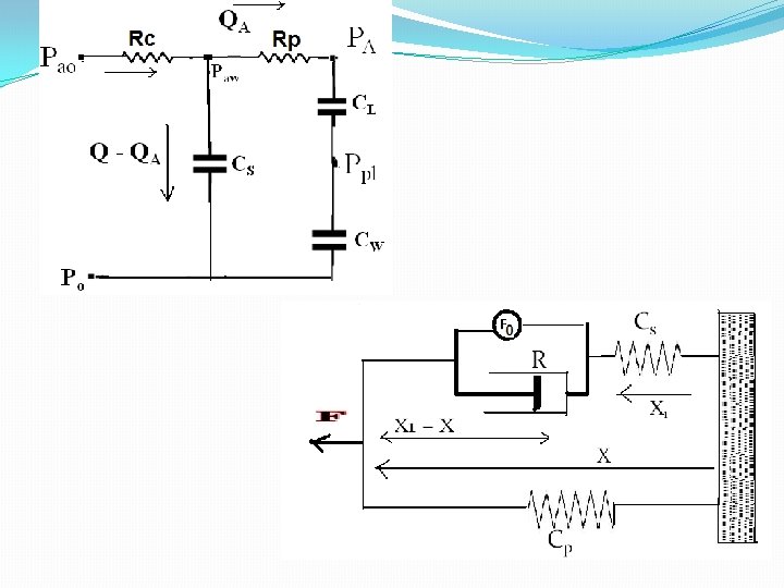
Linear model of respiratory mechanics �Airways- 1. larger / Central airways. = � 2. smaller / peripheral airways. = �CL & CW are the compliances of lung and chest wall, in series. �

Pao = Pressure at the airway opening. Q Paw = Pressure at the central airways. PA = Pressure in the alveoli. Ppl = Pressure in the pleural space (lung parenchyma & chest wall) Q = volume flow-rate of air entering the respiratory system. Q-QA = flow shunted away from the alveoli. Po = Reference pressure, ambient pressure.

�Applying Kirchoff’s first law to the closed circuit containing CS , RP , CL & C W. Applying Kirchoff’s first law to the closed circuit containing RC & CS.

�Differentiating both the equations with respect to time and reduce to one equations by eliminating QA.

MUSCLE MECHANICS

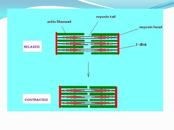
Muscle mechanics �Muscle is composed of a large number of muscle fibers. The muscle fibers are arranged in groups. Each group is under the control of a single motor neuron, the axon of which sends a terminal branch to each fiber of the group. All the muscle fibers of a group contract when a nerve impulse travels down their motor neuron.

Mechanism �A motor neuron and the group of muscle fibers innervated by its axon constitute a functional unit, called the motor unit. The number of muscle fiber and motor unit is variable and depends on the fineness of the control, a motor unit has to exercise. �Muscle fibers are composed of bundles of contractile muscle called myofibrils. Each myofibril is made up of smaller repeating units called sarcomeres. Thin filaments of actin and thick filaments of myosin form the muscle fibers.

Linear model of muscle mechanics. F 0 = force developed by the active contractile element of muscle. F= actual force of the muscle. R= viscous dampering of tissue. Cp = parallel elastic element. Cs=series elastic element. These reflects the storage properties of sarcolemma & muscle tendons.

�The force transmitted through Cs must be equal to the force transmitted through the parallel combination of F 0 & R, ------ 1 ------ 2 eliminating X 1 from above eqns yields the following differential eqn relating F,

�An isometric contraction of a muscle generates force without changing length. An example can be found when the muscles of the hand forearm grip an object; the joints of the hand do not move, but muscles generate sufficient force to prevent the object from being dropped.

Distributed parameter V/S Lumped Parameter model �Lumped parameter model: the property of the model is assumed to be concentrated into a single element. �Ex: Rc : trachea, branches of airway. �Cl : compliance of the lungs. � A distributed parameter model is a network of many small lumped-parameter sub-models. This model provides more realistic characterization of the spatial distribution.

Derivation of differential equation of a distributed-parameter model of the passive cable characteristics of an un-myelinated nerve fiber. Illustrates the relationship between distributed & lumped parameter model.

rx = axial resistance Cm = capacitance of nerve membrane. rm = resistance of nerve membrane.

�The increase of voltage δV occurring over an axial distance of δx is related to the axial current by: ------ 1 �The eqn bears a negative sign since the “increase” in voltage should be associated with a current flowing in a opposite direction. Divide both sides by δx & take limits. ------ 2

�The membrane current δI is related to the intracellular voltage V by: � Divide both sides by δx Finally, differentiate eqn 2 and substitute eqn 4 into eqn 2 :

This eqn is known as the one-dimensional cable eqn, and describes intracellular voltage along the nerve fiber as a continuous function of length and time.

LINEAR SYSTEMS & SUPERPOSITION PRINCIPLE

The general form of the differential eqn -----1 �The above eqn is of first order & linear. The coefficients a 1, a 2, b 0, b 1, b 2 are constant & timeinvariant. �Now make the eqn time variant, eg: x = x 1 (t) & y= y 1(t). It will be eqn 2 & again change the time course i. e, x as x 2 (t) & y = y 2 (t), it will be eqn 3. �

------ 2 �Add both the eqns 2 & 3

�Eqn 2 & 4 gives the response of as linear system of two different inputs. This results can be extended to more than two inputs and is known as “principle of superposition”.

The principle of superposition also implies that the complete solution( response in y) can be broken into two components, i. e �yc(t) = complementary function. �yp(t) = particular function. �In eqn 1, change y as yc(t), it is the response of the linear system and make input x(t)=0.

In eqn 1 change to, yp(t) is the response of the same linear system when the input x(t) is a particular function of time.

�yc(t) = the transient response & �yp(t) = the steady state response , when x(t) is an input forcing function that persists over time.

�LAPLACE TRANSFORMS AND TRANSFER FUNCTIONS.

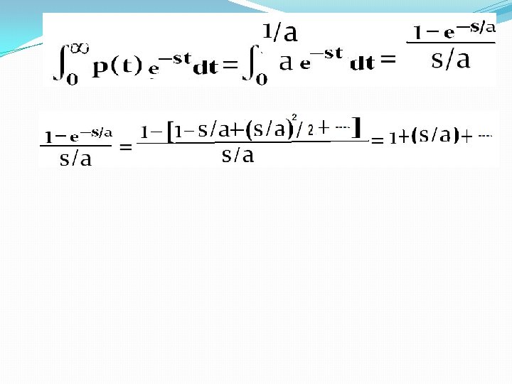
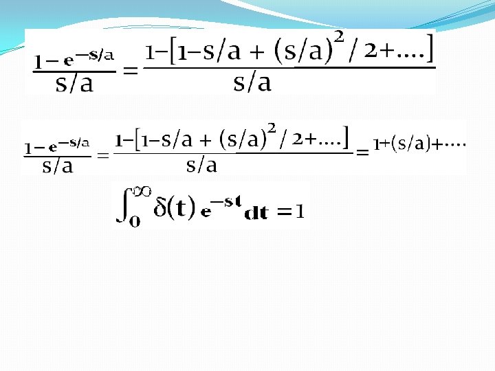
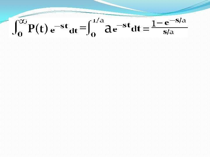
�The general form of the Laplace transformation: ---- 1 a �The inverse form is defined as: �---- 1 a ---- 1 b The laplace variable s is complex, i. e, s= σ + jω & j= √-1 �Differentiate the eqn 1 a: dy/dt:

---- 2 a �Thus, ---- 2 b By applying the same transformation to d 2 y/dt 2 , ---- 3

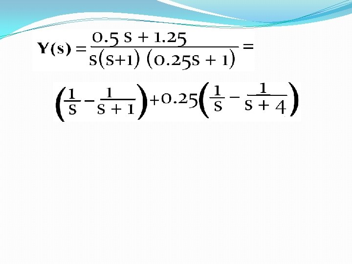
�Conversely, the laplace transform of the time integral of y(t), assuming y(t)=0 for t<0, is ---- 4 �By eqn 2 b & 3, get the first order eqn: ---- 5 a �In the above obtained eqn, x & y & their first time derivatives are all equal zero at time t=0. This eqn is rearranged and represented below. It gives the dynamic functional nature of the linear system.

---- 5 b �The ratio of Y(s) to X(s) is called the transfer function of the system.