Manipulative experiment Treatment It refers to the things

Manipulative experiment Treatment (處理) It refers to the things that are being compared e. g. drug 1 vs. drug 2 Experimental unit (實驗單位)/Experimental subjects (被實驗者) The basic unit that is exposed to the treatments e. g. patients, rats Response (反應) The random variable that is expected to be affected by treatments e. g. blood pressure, survival

Experimental design: independent samples f 1 m 2 m 3 m 1 f 2 m 1 m 4 f 2 m 2 f 4 m 3 f 3 f 4 m 4 f 1

Experimental design: paired samples – before vs after f 1 m 2 m 3 f 1 m 1 f 2 f 3 f 4 Before m 2 m 4 Drug 1 or 2 m 3 m 1 f 2 f 3 f 4 After m 4

Experimental design: paired samples – simultaneous testing f 1 m 2 Drug 1 m 3 m 1 f 2 f 3 f 4 m 4 Drug 2

Experimental design: paired samples – block design f 1 m 2 m 3 m 1 f 2 m 4 f 1 m 3 f 4 m 2 f 2 m 1 f 3 Pair 1 Pair 2 Pair 3 Pair 4 f 3 f 4 m 4 Match for gender height weight age

Commonly used experimental designs Independent samples (Complete randomization) Paired samples

Analysis of Variance (ANOVA) Compare means of multiple populations More than two populations: ANOVA Two populations: ANOVA or two-sample t test The null and alternative hypotheses are: at least one pair of μ’s is not equal

ANOVA assumptions Ø The k samples represent independent random samples drawn from k populations with means μ 1, μ 2, . . , μk. Ø Each of the k populations is normally distributed Ø The k populations have the same variance, This is called “homogeneity of variance” assumption (recall the equal variance assumption in two-sample t test)

Does diet affect lifespan? What are the null and alternative hypotheses? What are the treatments? What are the response variables? What are the experimental units? Are experimental units randomly assigned to the treatments? Unlimited 90% diet 80% diet

Unlimited 90% diet 80% diet 2. 5 2. 7 3. 1 2. 9 i = 1, 2, …, k 2. 3 2. 9 3. 8 j = 1, 2, …, n 1. 9 3. 7 3. 9 2. 4 3. 5 4. 0

Deviation The deviation of an observation from the grand mean can be partitioned into two components: Deviation from an observation to the grand mean Deviation from the group mean to the grand mean Deviation from an observation to its group mean

Sums of Squares (SS) Total variability across all observations and treatments: Total Sums of Squares or SSTotal

=0

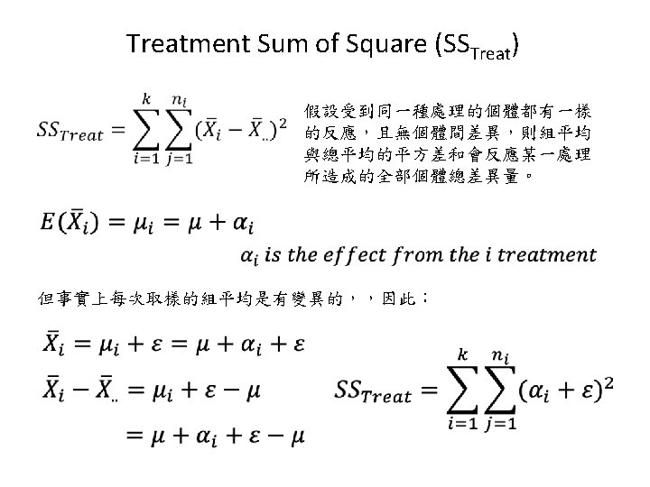
Among treatment SS Residual SS Explained variability Unexplained variability Explained by the treatment, or group membership

i = 1, 2, 3 (k = 3) Unlimited (i =1) 90% diet (i =2) 80% diet (i =3) 2. 5 2. 7 3. 1 2. 9 2. 3 2. 9 3. 8 1. 9 3. 7 3. 9 2. 4 3. 5 4. 0 j = 1, . . , 5 (n = 5)

i = 1, 2, 3 (k = 3) Unlimited (i =1) 90% diet (i =2) 80% diet (i =3) 2. 5 2. 7 3. 1 2. 9 2. 3 2. 9 3. 8 1. 9 3. 7 3. 9 2. 4 3. 5 4. 0 j = 1, . . , 5 (n = 5)

i = 1, 2, 3 (k = 3) Unlimited (i =1) 90% diet (i =2) 80% diet (i =3) 2. 5 2. 7 3. 1 2. 9 2. 3 2. 9 3. 8 1. 9 3. 7 3. 9 2. 4 3. 5 4. 0 j = 1, . . , 5 (n = 5)

i = 1, 2, 3 (k = 3) Unlimited (i =1) 90% diet (i =2) 80% diet (i =3) 2. 5 2. 7 3. 1 2. 9 2. 3 2. 9 3. 8 1. 9 3. 7 3. 9 2. 4 3. 5 4. 0 j = 1, . . , 5 (n = 5)

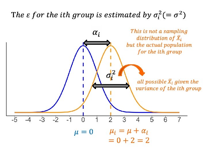
Homogeneity of variance = … … = = … = This is the group variance common to all k treatments =

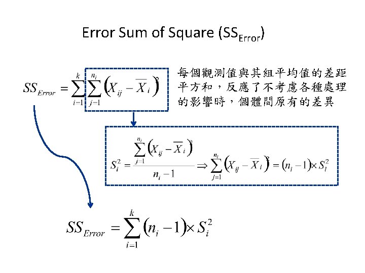
Error Sums of Squares (SSError)

Error Mean Square (MSError)

Treatment Mean Square (MSTreat) Also see Appendix A 3 and A 4 in the textbook for the algebraic proof The weighted average of among-group variance

ANOVA: F test Under the null hypothesis and assuming equal variance =0 If the null hypothesis IS NOT TRUE, we would expect: >0

Degree of freedom Similar to how we partition the sums of squares, we can partition the degree of freedom into treatment DF and error DF

F distributions density F

One-way ANOVA comparing mouse lifespan ANOVA Table:

density F 2, 12 = 7. 70 F The probability of getting a F ≥ 7. 7 is 0. 007 Diet has a significant effect on mouse life span (F 2, 12 = 7. 70, P = 0. 007).

Multiple Comparisons The F test that we performed is also called global F test. A global F test is often followed by multiple comparisons if the null hypothesis is rejected. When we confirmed that at least one pair of the means is not equal, we would often like to find out which pairs do not have equal means.

Type I error inflation If there are k treatments, we will have pairwise comparisons. For mouse lifespan data, we have three pairwise comparisons:

Type I error inflation What is Type I error (α)? The probability of rejecting a correct null hypothesis. What is 1 – α? The probability of accepting a correct null hypothesis.

Type I error inflation If we have a probability of 0. 95 (1 -α) to accept the correct null hypothesis in each of the three tests, the probability of accepting all three correct hypotheses: and the probability of rejecting any one of the three correct hypotheses: > 0. 05 By doing multiple t tests, Type I error is inflated.

Experiment-wise Type I error In order to control the overall or experiment-wise Type I error (α´), we need to adjust α level in each test. Bonferroni adjustment: For three pairs of comparisons:

Multiple comparisons with Bonferroni adjusted Type I error • The mice had a significantly shorter life span when fed unlimited diet compared to 80% diet (Bonferroni-adjusted P = 0. 007). • The mice also tended to have a shorter life span when fed unlimited diet compared to 90% diet, with a marginal significance (Bonferroni-adjusted, P = 0. 07). • There was no difference in life span between the mice on 80% and 905 diets (Bonferroniadjusted, P = 0. 7). Different letters indicate the group means are statistically different.