Linear Filters Devi Parikh Disclaimer Many slides have

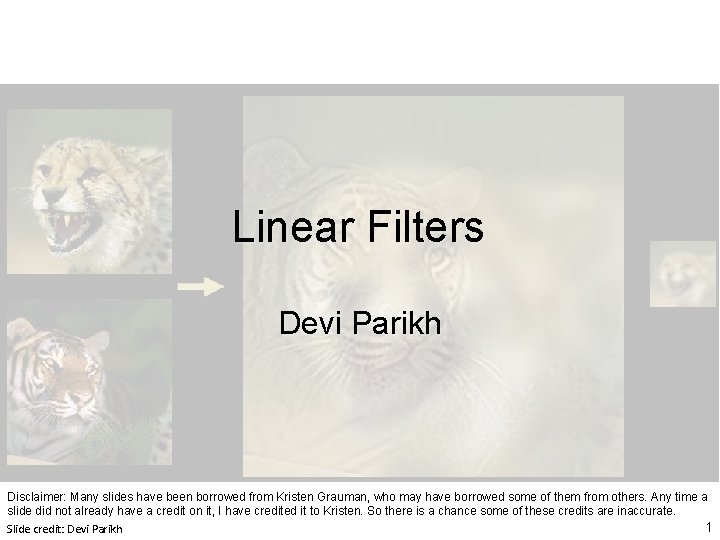
Linear Filters Devi Parikh Disclaimer: Many slides have been borrowed from Kristen Grauman, who may have borrowed some of them from others. Any time a slide did not already have a credit on it, I have credited it to Kristen. So there is a chance some of these credits are inaccurate. 1 Slide credit: Devi Parikh

Announcements • PS 0 due Monday at 11: 58: 59 pm • Start thinking about project teams Slide credit: Devi Parikh 2

Topics overview • • • Intro Features & filters Grouping & fitting Multiple views and motion Recognition Video processing Slide credit: Kristen Grauman 3

Topics overview • • • Intro Features & filters Grouping & fitting Multiple views and motion Recognition Video processing Slide credit: Kristen Grauman 4

Topics overview • • • Intro Features & filters Grouping & fitting Multiple views and motion Recognition Video processing Slide credit: Kristen Grauman 5

Topics overview • Intro • Features & filters – Filters • • Grouping & fitting Multiple views and motion Recognition Video processing Slide credit: Kristen Grauman 6

Topics overview • Intro • Features & filters – Filters • • Grouping & fitting Multiple views and motion Recognition Video processing Neat interactive tool: http: //setosa. io/ev/image-kernels/ (thanks to Michael Cogswell) Slide credit: Kristen Grauman 7

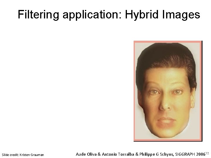
Plan for today • Image formation • Image noise • Linear filters – Examples: smoothing filters • Convolution / correlation • Cool application: hybrid images Slide credit: Modified from Kristen Grauman 8

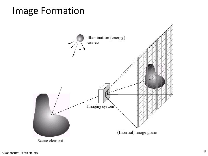
Image Formation Slide credit: Derek Hoiem 9

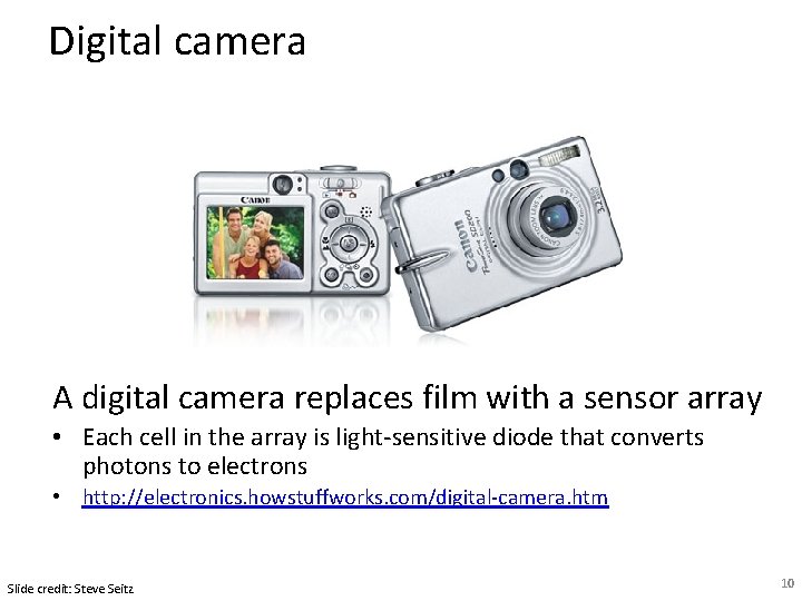
Digital camera A digital camera replaces film with a sensor array • Each cell in the array is light-sensitive diode that converts photons to electrons • http: //electronics. howstuffworks. com/digital-camera. htm Slide credit: Steve Seitz 10

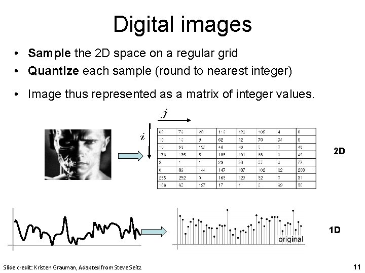
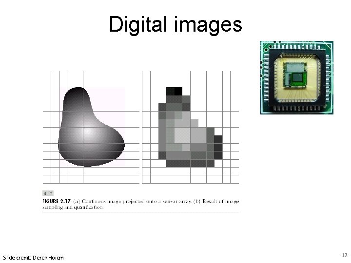
Digital images • Sample the 2 D space on a regular grid • Quantize each sample (round to nearest integer) • Image thus represented as a matrix of integer values. 2 D 1 D Slide credit: Kristen Grauman, Adapted from Steve Seitz 11

Digital images Slide credit: Derek Hoiem 12

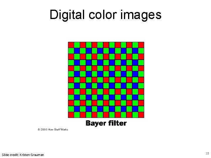
Digital color images Slide credit: Kristen Grauman 13

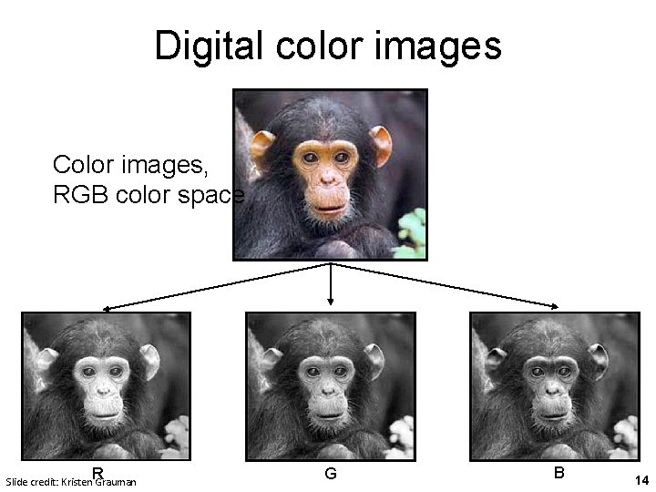
Digital color images Color images, RGB color space R Slide credit: Kristen Grauman G B 14

Image filtering • Compute a function of the local neighborhood at each pixel in the image – Function specified by a “filter” or mask saying how to combine values from neighbors. • Uses of filtering: – Enhance an image (denoise, resize, etc) – Extract information (texture, edges, etc) – Detect patterns (template matching) Slide credit: Kristen Grauman, Adapted from Derek Hoiem 16

Image filtering • Compute a function of the local neighborhood at each pixel in the image – Function specified by a “filter” or mask saying how to combine values from neighbors. • Uses of filtering: – Enhance an image (denoise, resize, etc) – Extract information (texture, edges, etc) – Detect patterns (template matching) Slide credit: Kristen Grauman, Adapted from Derek Hoiem 17

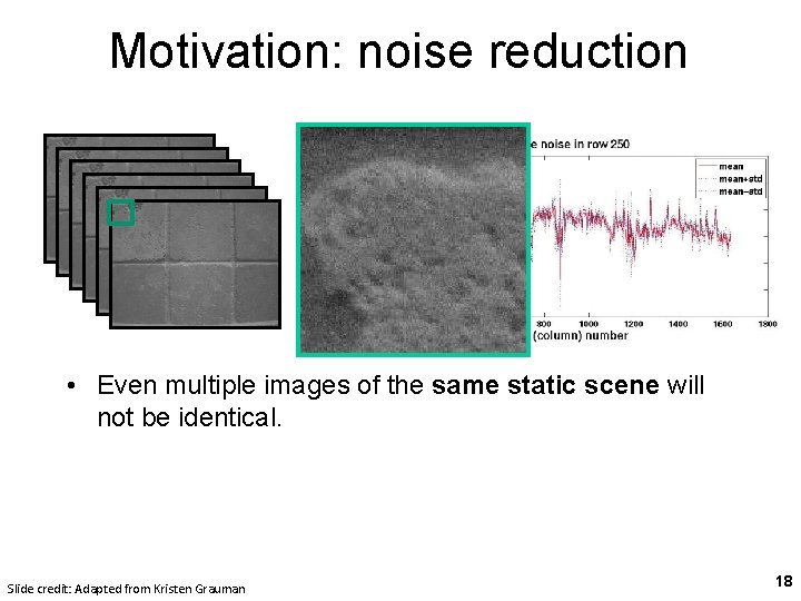
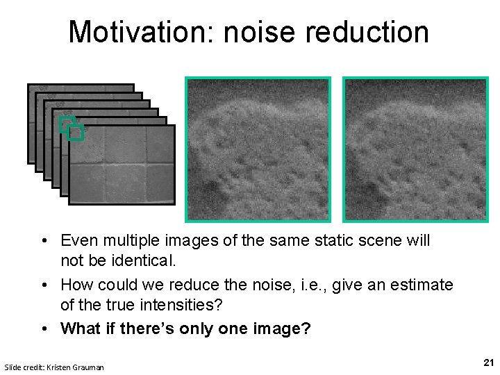
Motivation: noise reduction • Even multiple images of the same static scene will not be identical. Slide credit: Adapted from Kristen Grauman 18

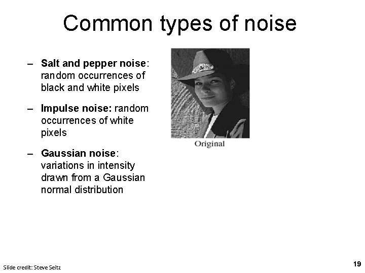
Common types of noise – Salt and pepper noise: random occurrences of black and white pixels – Impulse noise: random occurrences of white pixels – Gaussian noise: variations in intensity drawn from a Gaussian normal distribution Slide credit: Steve Seitz 19

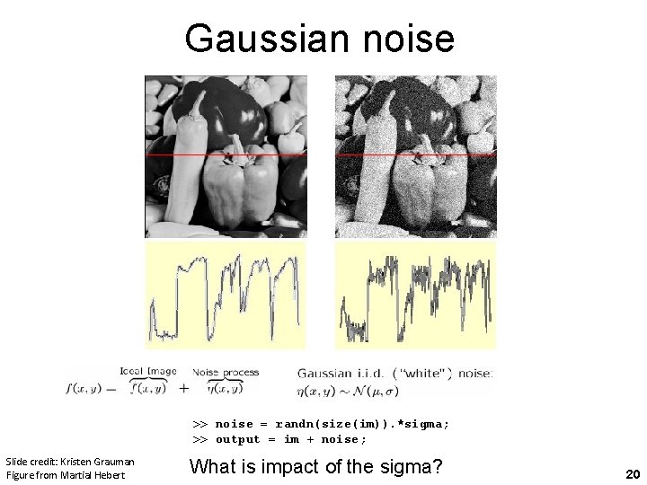
Gaussian noise >> noise = randn(size(im)). *sigma; >> output = im + noise; Slide credit: Kristen Grauman Figure from Martial Hebert What is impact of the sigma? 20

Motivation: noise reduction • Even multiple images of the same static scene will not be identical. • How could we reduce the noise, i. e. , give an estimate of the true intensities? • What if there’s only one image? Slide credit: Kristen Grauman 21

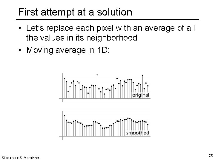
First attempt at a solution • Let’s replace each pixel with an average of all the values in its neighborhood • Assumptions: • Expect pixels to be like their neighbors • Expect noise processes to be independent from pixel to pixel Slide credit: Kristen Grauman 22

First attempt at a solution • Let’s replace each pixel with an average of all the values in its neighborhood • Moving average in 1 D: Slide credit: S. Marschner 23

Weighted Moving Average Can add weights to our moving average Weights [1, 1, 1] / 5 Slide credit: S. Marschner 24

Weighted Moving Average Non-uniform weights [1, 4, 6, 4, 1] / 16 Slide credit: S. Marschner 25

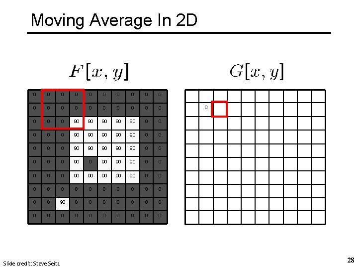
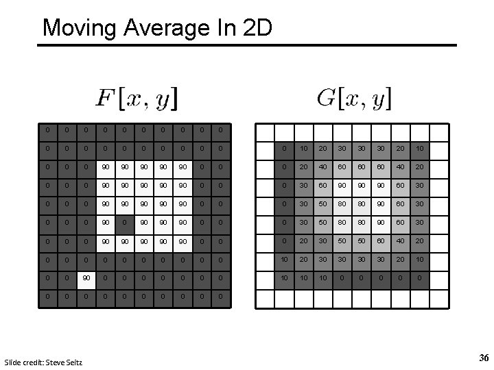
Moving Average In 2 D 0 0 0 0 0 0 90 90 90 0 0 90 90 90 0 90 90 90 0 0 0 0 0 0 0 0 0 0 Slide credit: Steve Seitz 26

Moving Average In 2 D 0 0 0 0 0 0 90 90 90 0 0 90 90 90 0 90 90 90 0 0 0 0 0 0 0 0 0 0 Slide credit: Steve Seitz 0 27

Moving Average In 2 D 0 0 0 0 0 0 90 90 90 0 0 90 90 90 0 90 90 90 0 0 0 0 0 0 0 0 0 0 Slide credit: Steve Seitz 0 28

Moving Average In 2 D 0 0 0 0 0 0 90 90 90 0 0 90 90 90 0 90 90 90 0 0 0 0 0 0 0 0 0 0 Slide credit: Steve Seitz 0 10 29

Moving Average In 2 D 0 0 0 0 0 0 90 90 90 0 0 90 90 90 0 90 90 90 0 0 0 0 0 0 0 0 0 0 Slide credit: Steve Seitz 0 10 30

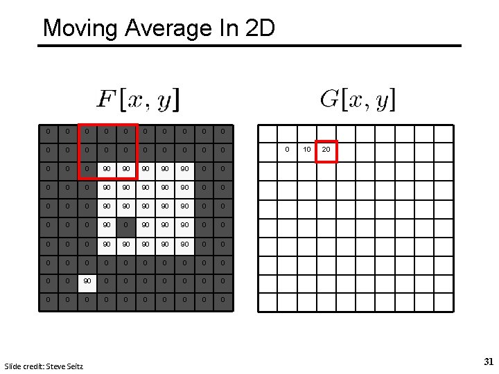
Moving Average In 2 D 0 0 0 0 0 0 90 90 90 0 0 90 90 90 0 90 90 90 0 0 0 0 0 0 0 0 0 0 Slide credit: Steve Seitz 0 10 20 31

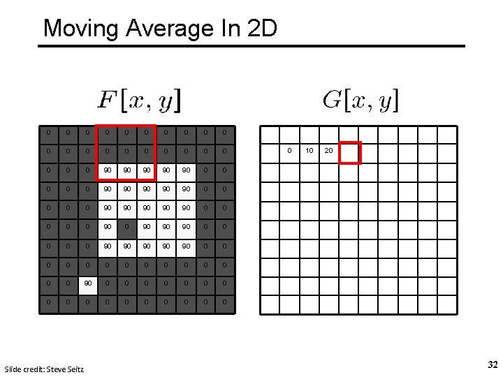
Moving Average In 2 D 0 0 0 0 0 0 90 90 90 0 0 90 90 90 0 90 90 90 0 0 0 0 0 0 0 0 0 0 Slide credit: Steve Seitz 0 10 20 32

Moving Average In 2 D 0 0 0 0 0 0 90 90 90 0 0 90 90 90 0 90 90 90 0 0 0 0 0 0 0 0 0 0 Slide credit: Steve Seitz 0 10 20 30 33

Moving Average In 2 D 0 0 0 0 0 0 90 90 90 0 0 90 90 90 0 90 90 90 0 0 0 0 0 0 0 0 0 0 Slide credit: Steve Seitz 0 10 20 30 34

Moving Average In 2 D 0 0 0 0 0 0 90 90 90 0 0 90 90 90 0 90 90 90 0 0 0 0 0 0 0 0 0 0 Slide credit: Steve Seitz 0 10 20 30 30 35

Moving Average In 2 D 0 0 0 0 0 0 10 20 30 30 30 20 10 0 90 90 90 0 20 40 60 60 60 40 20 0 90 90 90 0 30 60 90 90 90 60 30 0 90 90 90 0 30 50 80 80 90 60 30 0 90 90 90 0 20 30 50 50 60 40 20 0 0 10 20 30 30 20 10 0 0 90 0 0 0 10 10 10 0 0 0 Slide credit: Steve Seitz 36

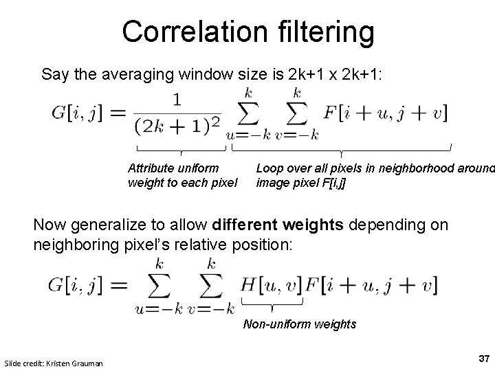
Correlation filtering Say the averaging window size is 2 k+1 x 2 k+1: Attribute uniform weight to each pixel Loop over all pixels in neighborhood around image pixel F[i, j] Now generalize to allow different weights depending on neighboring pixel’s relative position: Non-uniform weights Slide credit: Kristen Grauman 37

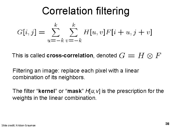
Correlation filtering This is called cross-correlation, denoted Filtering an image: replace each pixel with a linear combination of its neighbors. The filter “kernel” or “mask” H[u, v] is the prescription for the weights in the linear combination. Slide credit: Kristen Grauman 38

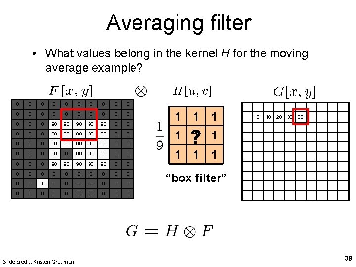
Averaging filter • What values belong in the kernel H for the moving average example? 0 0 0 0 0 0 90 90 90 0 0 90 90 90 0 90 90 90 0 0 0 0 0 0 0 0 0 0 Slide credit: Kristen Grauman 1 1 1 0 10 20 30 30 ? 1 1 1 “box filter” 39

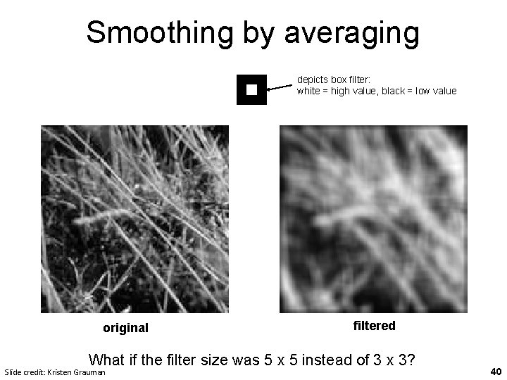
Smoothing by averaging depicts box filter: white = high value, black = low value original filtered What if the filter size was 5 x 5 instead of 3 x 3? Slide credit: Kristen Grauman 40

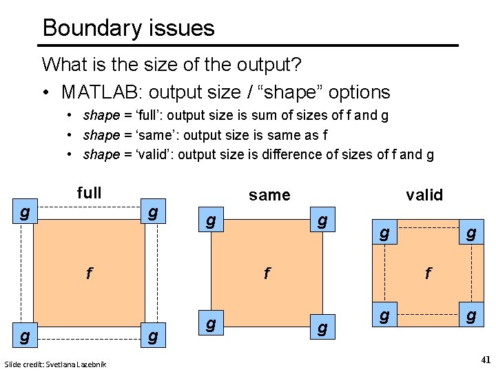
Boundary issues What is the size of the output? • MATLAB: output size / “shape” options • shape = ‘full’: output size is sum of sizes of f and g • shape = ‘same’: output size is same as f • shape = ‘valid’: output size is difference of sizes of f and g full g g same g f g Slide credit: Svetlana Lazebnik valid g g f g g g 41

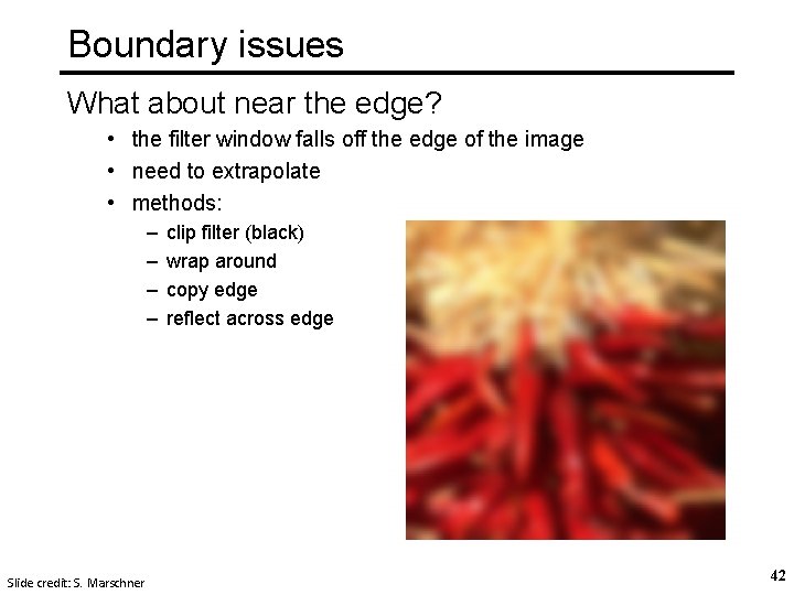
Boundary issues What about near the edge? • the filter window falls off the edge of the image • need to extrapolate • methods: – – Slide credit: S. Marschner clip filter (black) wrap around copy edge reflect across edge 42

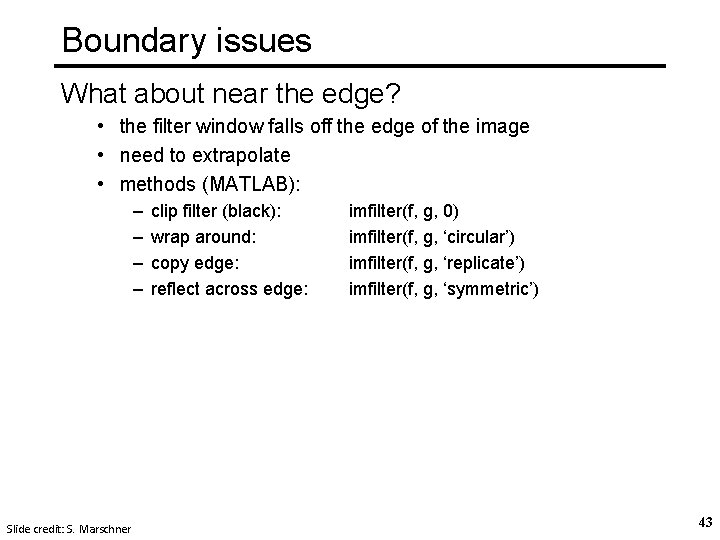
Boundary issues What about near the edge? • the filter window falls off the edge of the image • need to extrapolate • methods (MATLAB): – – Slide credit: S. Marschner clip filter (black): wrap around: copy edge: reflect across edge: imfilter(f, g, 0) imfilter(f, g, ‘circular’) imfilter(f, g, ‘replicate’) imfilter(f, g, ‘symmetric’) 43

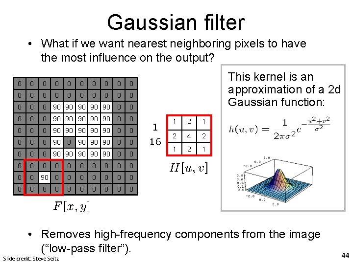
Gaussian filter • What if we want nearest neighboring pixels to have the most influence on the output? 0 0 0 0 0 0 90 90 90 0 0 90 90 90 0 90 90 90 0 0 0 0 0 0 0 0 0 0 This kernel is an approximation of a 2 d Gaussian function: 1 2 4 2 1 • Removes high-frequency components from the image (“low-pass filter”). Slide credit: Steve Seitz 44

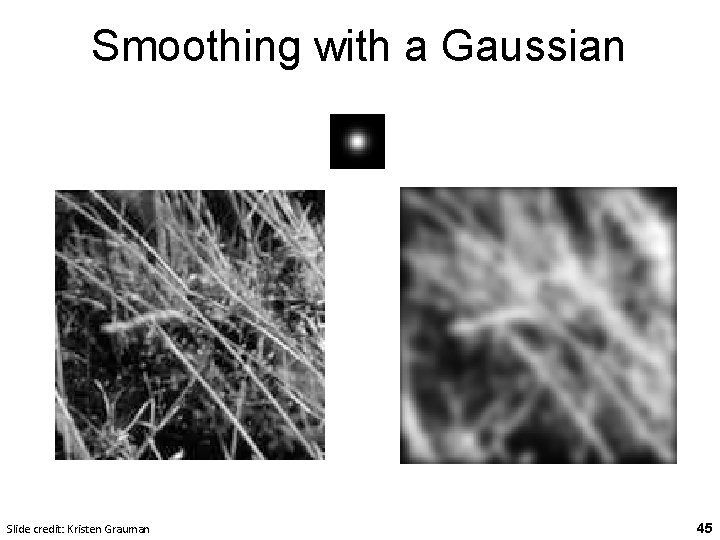
Smoothing with a Gaussian Slide credit: Kristen Grauman 45

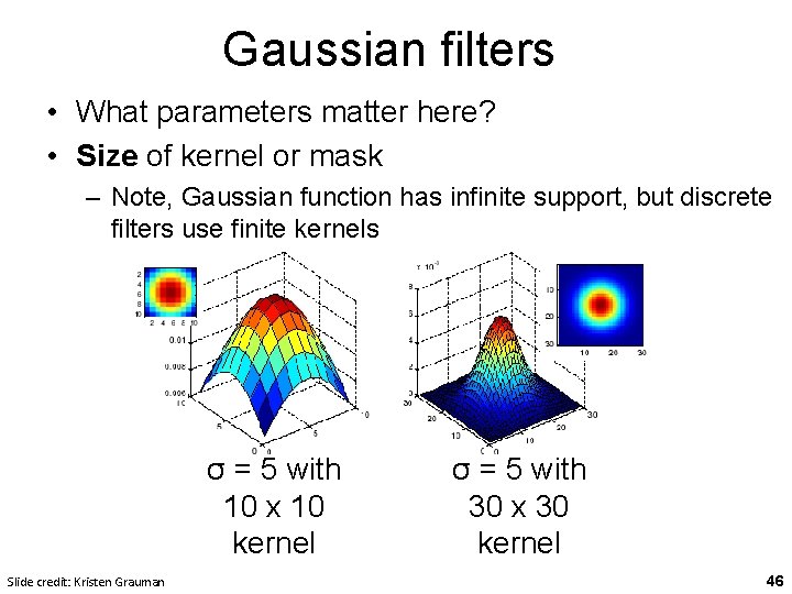
Gaussian filters • What parameters matter here? • Size of kernel or mask – Note, Gaussian function has infinite support, but discrete filters use finite kernels σ = 5 with 10 x 10 kernel Slide credit: Kristen Grauman σ = 5 with 30 x 30 kernel 46

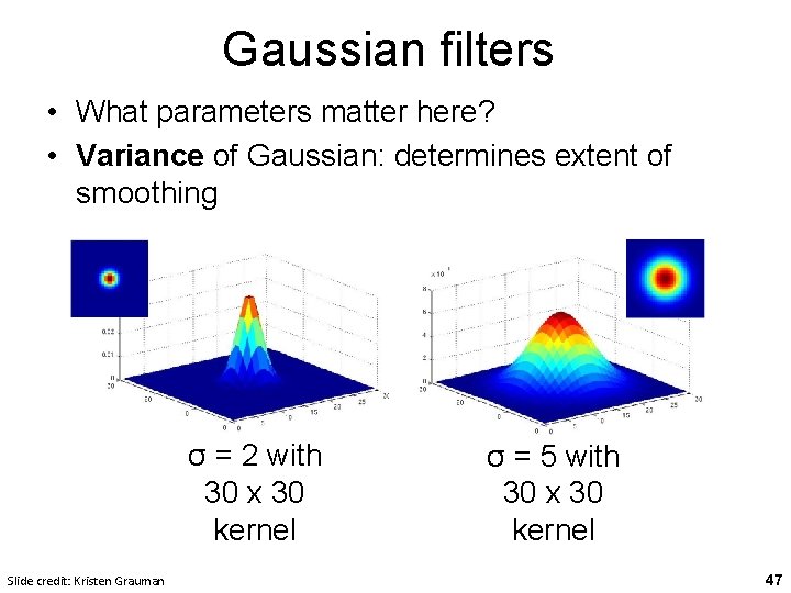
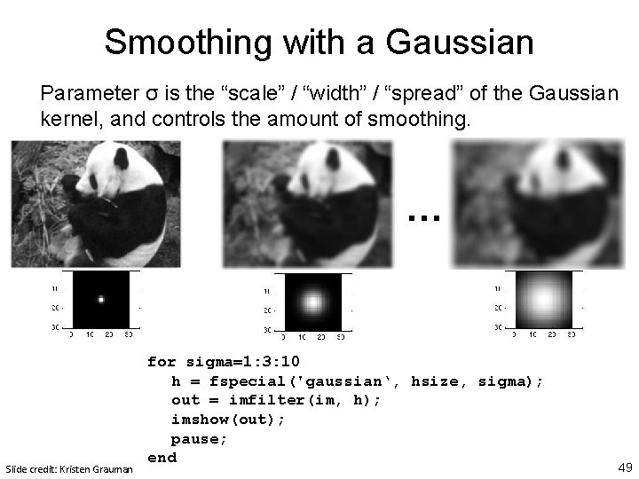
Gaussian filters • What parameters matter here? • Variance of Gaussian: determines extent of smoothing σ = 2 with 30 x 30 kernel Slide credit: Kristen Grauman σ = 5 with 30 x 30 kernel 47

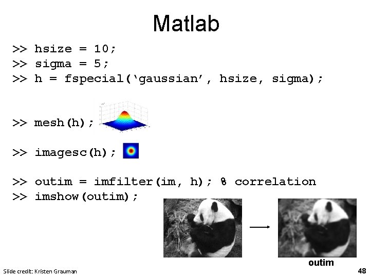
Matlab >> hsize = 10; >> sigma = 5; >> h = fspecial(‘gaussian’, hsize, sigma); >> mesh(h); >> imagesc(h); >> outim = imfilter(im, h); % correlation >> imshow(outim); Slide credit: Kristen Grauman outim 48

Smoothing with a Gaussian Parameter σ is the “scale” / “width” / “spread” of the Gaussian kernel, and controls the amount of smoothing. … Slide credit: Kristen Grauman for sigma=1: 3: 10 h = fspecial('gaussian‘, hsize, sigma); out = imfilter(im, h); imshow(out); pause; end 49

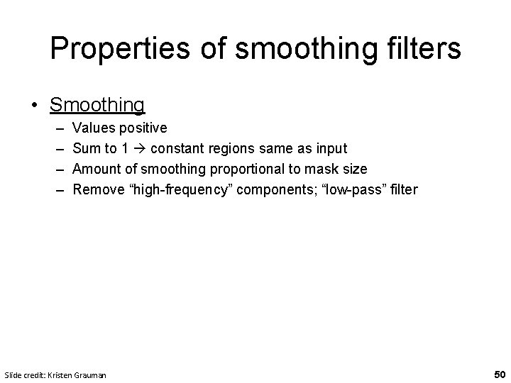
Properties of smoothing filters • Smoothing – – Values positive Sum to 1 constant regions same as input Amount of smoothing proportional to mask size Remove “high-frequency” components; “low-pass” filter Slide credit: Kristen Grauman 50

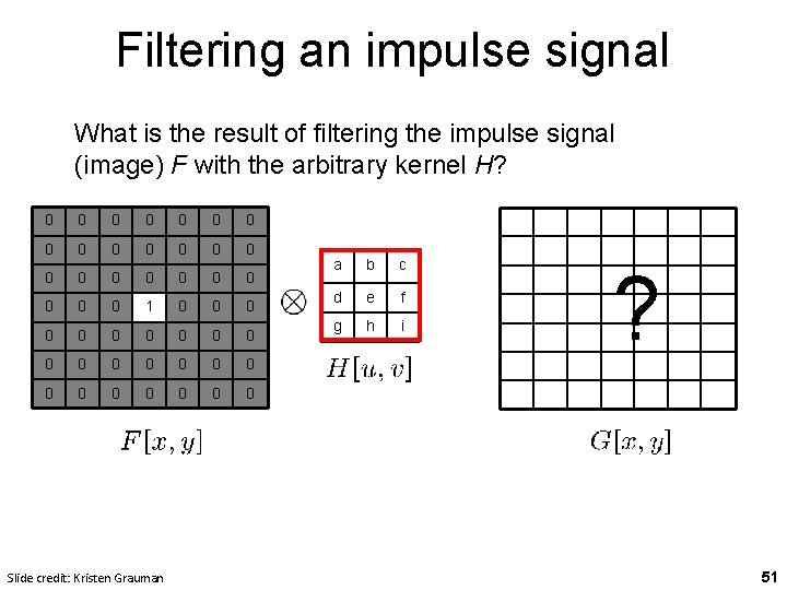
Filtering an impulse signal What is the result of filtering the impulse signal (image) F with the arbitrary kernel H? 0 0 0 0 0 0 1 0 0 0 0 0 0 Slide credit: Kristen Grauman a b c d e f g h i ? 51

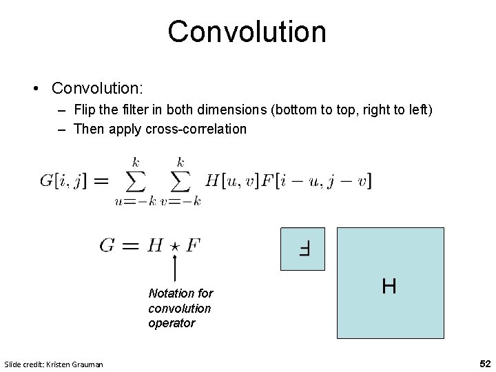
Convolution • Convolution: – Flip the filter in both dimensions (bottom to top, right to left) – Then apply cross-correlation F Notation for convolution operator Slide credit: Kristen Grauman H 52

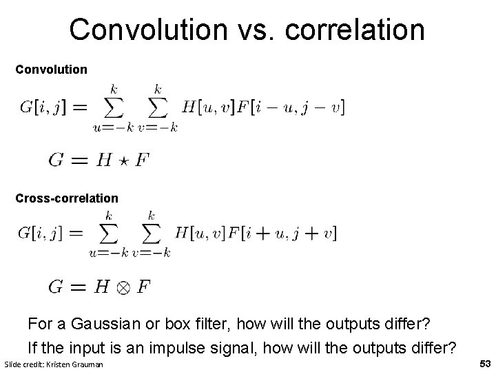
Convolution vs. correlation Convolution Cross-correlation For a Gaussian or box filter, how will the outputs differ? If the input is an impulse signal, how will the outputs differ? Slide credit: Kristen Grauman 53

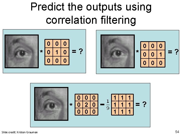
Predict the outputs using correlation filtering * 0 0 1 0 0 =? * Slide credit: Kristen Grauman 0 0 2 0 0 * - 1 1 1 1 1 0 0 0 =? 54

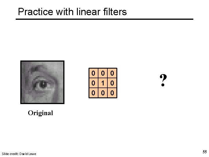
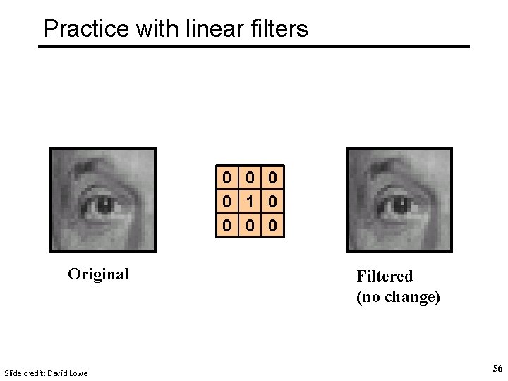
Practice with linear filters 0 0 1 0 0 ? Original Slide credit: David Lowe 55

Practice with linear filters 0 0 1 0 0 Original Slide credit: David Lowe Filtered (no change) 56

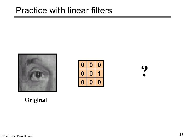
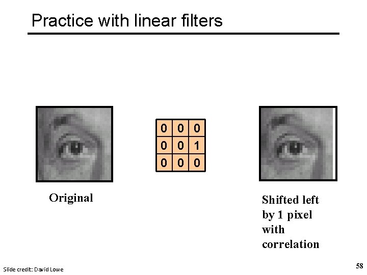
Practice with linear filters 0 0 0 1 0 0 0 ? Original Slide credit: David Lowe 57

Practice with linear filters 0 0 0 1 0 0 0 Original Slide credit: David Lowe Shifted left by 1 pixel with correlation 58

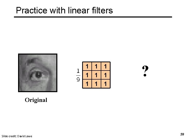
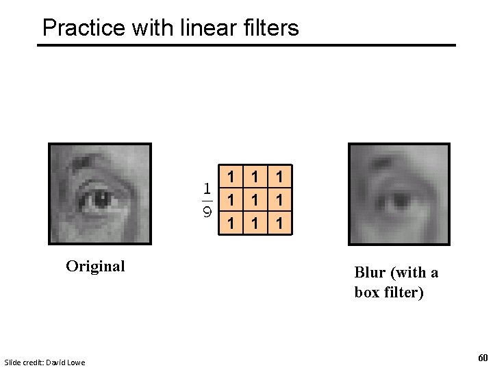
Practice with linear filters 1 1 1 1 1 ? Original Slide credit: David Lowe 59

Practice with linear filters 1 1 1 1 1 Original Slide credit: David Lowe Blur (with a box filter) 60

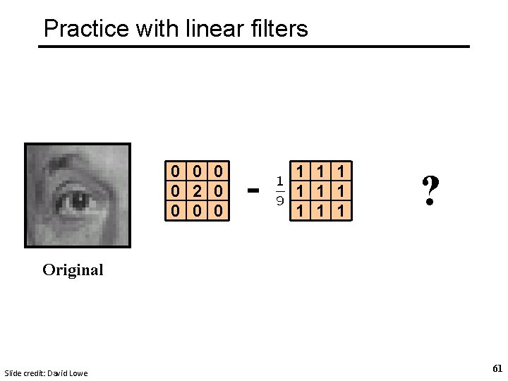
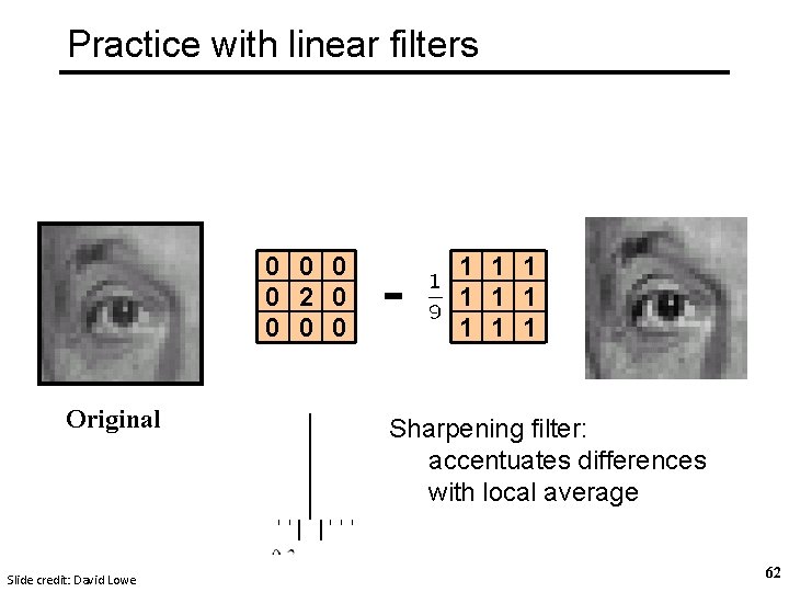
Practice with linear filters 0 0 2 0 0 - 1 1 1 1 1 ? Original Slide credit: David Lowe 61

Practice with linear filters 0 0 2 0 0 Original Slide credit: David Lowe - 1 1 1 1 1 Sharpening filter: accentuates differences with local average 62

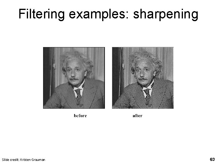
Filtering examples: sharpening Slide credit: Kristen Grauman 63

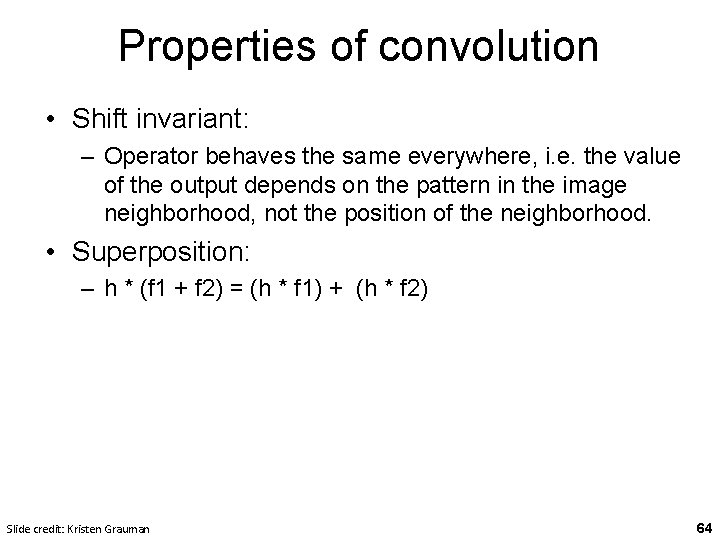
Properties of convolution • Shift invariant: – Operator behaves the same everywhere, i. e. the value of the output depends on the pattern in the image neighborhood, not the position of the neighborhood. • Superposition: – h * (f 1 + f 2) = (h * f 1) + (h * f 2) Slide credit: Kristen Grauman 64

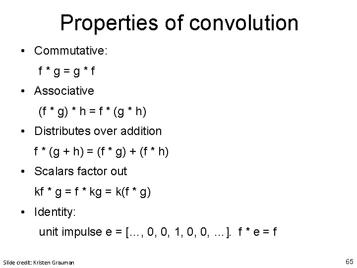
Properties of convolution • Commutative: f*g=g*f • Associative (f * g) * h = f * (g * h) • Distributes over addition f * (g + h) = (f * g) + (f * h) • Scalars factor out kf * g = f * kg = k(f * g) • Identity: unit impulse e = […, 0, 0, 1, 0, 0, …]. f * e = f Slide credit: Kristen Grauman 65

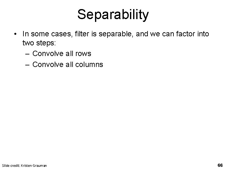
Separability • In some cases, filter is separable, and we can factor into two steps: – Convolve all rows – Convolve all columns Slide credit: Kristen Grauman 66

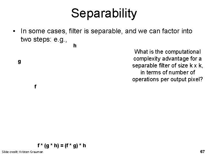
Separability • In some cases, filter is separable, and we can factor into two steps: e. g. , h What is the computational complexity advantage for a separable filter of size k x k, in terms of number of operations per output pixel? g f f * (g * h) = (f * g) * h Slide credit: Kristen Grauman 67

Effect of smoothing filters Additive Gaussian noise Slide credit: Kristen Grauman Salt and pepper noise 68

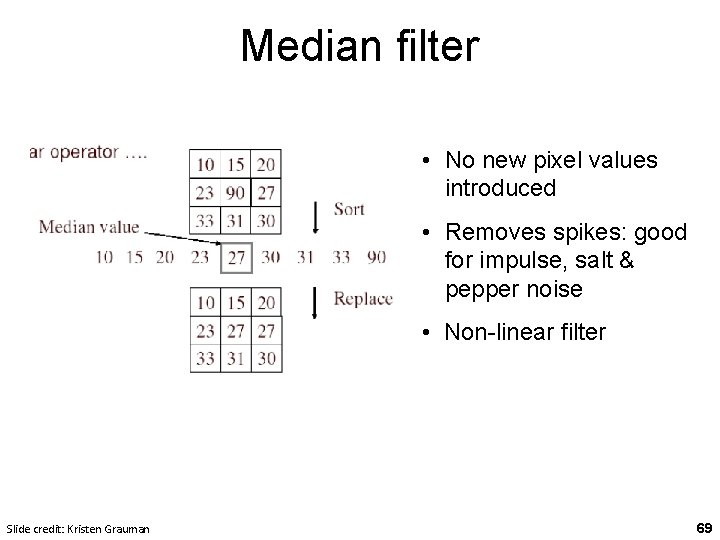
Median filter • No new pixel values introduced • Removes spikes: good for impulse, salt & pepper noise • Non-linear filter Slide credit: Kristen Grauman 69

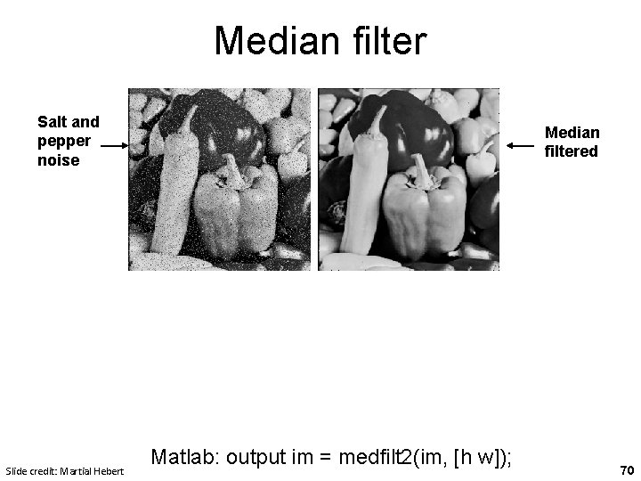
Median filter Salt and pepper noise Median filtered Plots of a row of the image Slide credit: Martial Hebert Matlab: output im = medfilt 2(im, [h w]); 70

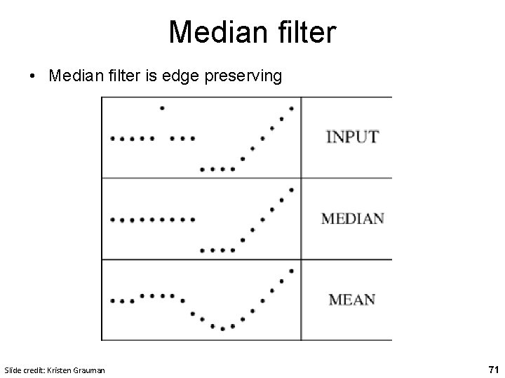
Median filter • Median filter is edge preserving Slide credit: Kristen Grauman 71

Filtering application: Hybrid Images Slide credit: Kristen Grauman Aude Oliva & Antonio Torralba & Philippe G Schyns, SIGGRAPH 200672

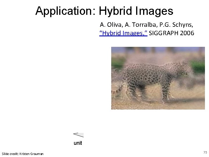
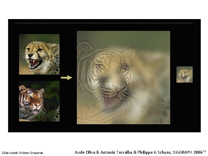
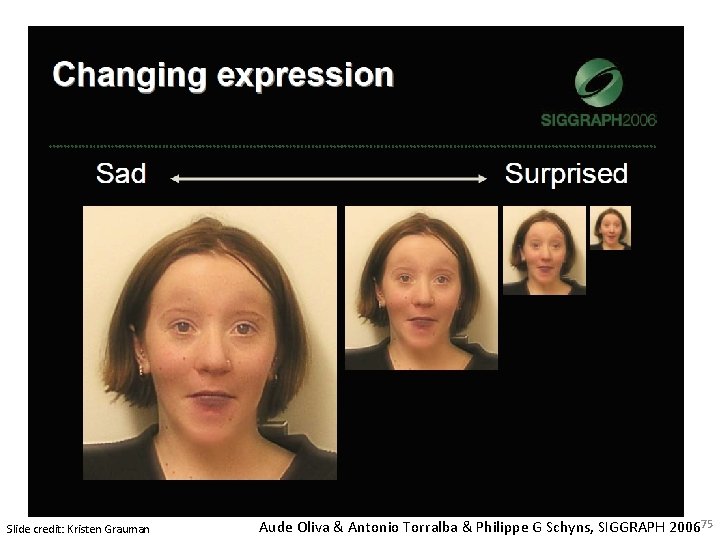
Application: Hybrid Images Gaussian Filter A. Oliva, A. Torralba, P. G. Schyns, “Hybrid Images, ” SIGGRAPH 2006 Laplacian Filter unit impulse Slide credit: Kristen Grauman Gaussian Laplacian of Gaussian 73

Slide credit: Kristen Grauman Aude Oliva & Antonio Torralba & Philippe G Schyns, SIGGRAPH 200674

Slide credit: Kristen Grauman Aude Oliva & Antonio Torralba & Philippe G Schyns, SIGGRAPH 200675

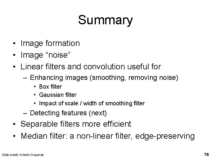
Summary • Image formation • Image “noise” • Linear filters and convolution useful for – Enhancing images (smoothing, removing noise) • Box filter • Gaussian filter • Impact of scale / width of smoothing filter – Detecting features (next) • Separable filters more efficient • Median filter: a non-linear filter, edge-preserving Slide credit: Kristen Grauman 76

Topics overview • Intro • Features & filters – Filters – Gradients – Edges • • Grouping & fitting Multiple views and motion Recognition Video processing Slide credit: Kristen Grauman 77

Questions?