Local features detection and description Devi Parikh Disclaimer

Local features: detection and description Devi Parikh Disclaimer: Most slides have been borrowed from Kristen Grauman, who may have borrowed some of them from others. Any time a slide did not already have a credit on it, I have credited it to Kristen. So there is a chance some of these credits are inaccurate. Slide credit: Kristen Grauman 1

Topics overview • • Intro Features & filters Grouping & fitting Multiple views and motion – – – Homography and image warping Local invariant features Image formation Epipolar geometry Stereo and structure from motion • Recognition • Video processing Slide credit: Kristen Grauman 2

Last time • Detecting corner-like points in an image Slide credit: Kristen Grauman 3

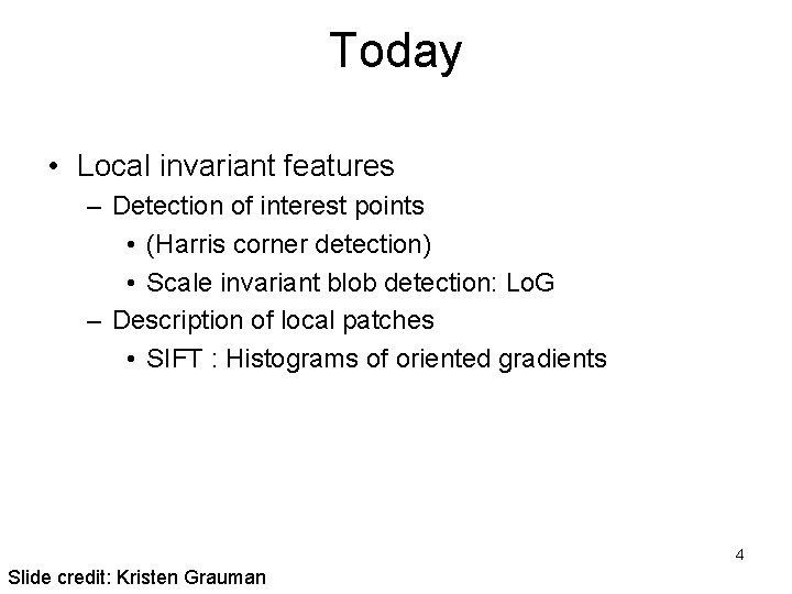
Today • Local invariant features – Detection of interest points • (Harris corner detection) • Scale invariant blob detection: Lo. G – Description of local patches • SIFT : Histograms of oriented gradients 4 Slide credit: Kristen Grauman

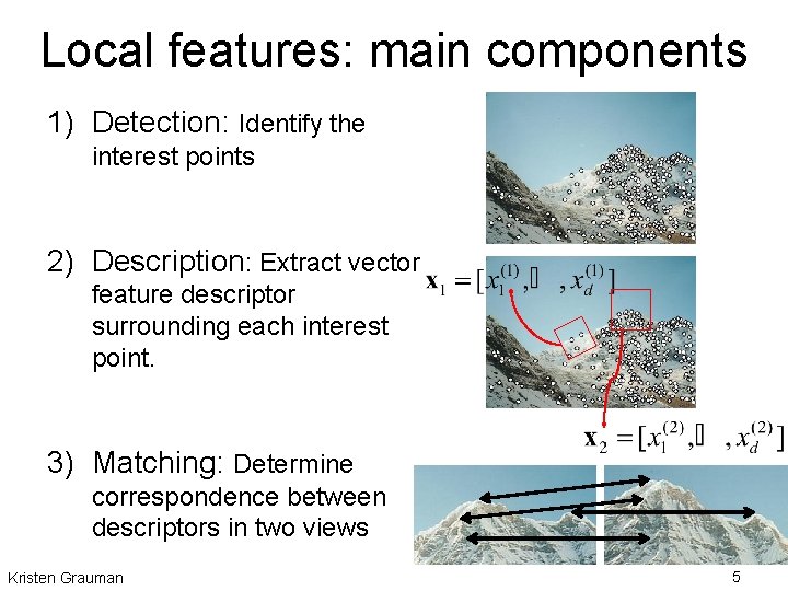
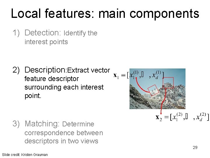
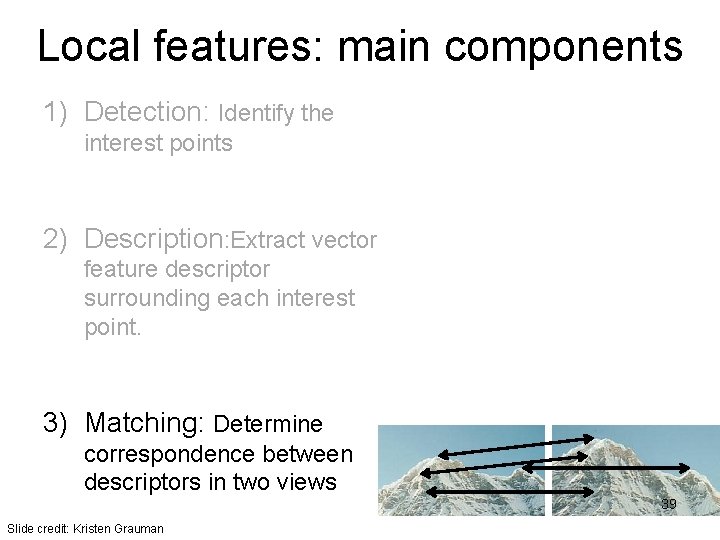
Local features: main components 1) Detection: Identify the interest points 2) Description: Extract vector feature descriptor surrounding each interest point. 3) Matching: Determine correspondence between descriptors in two views Kristen Grauman 5

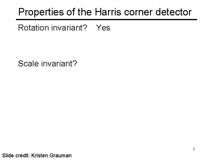
Properties of the Harris corner detector Rotation invariant? Yes Scale invariant? 7 Slide credit: Kristen Grauman

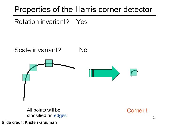
Properties of the Harris corner detector Rotation invariant? Scale invariant? All points will be classified as edges Slide credit: Kristen Grauman Yes No Corner ! 8

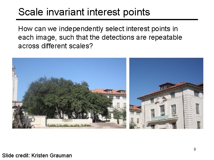
Scale invariant interest points How can we independently select interest points in each image, such that the detections are repeatable across different scales? 9 Slide credit: Kristen Grauman

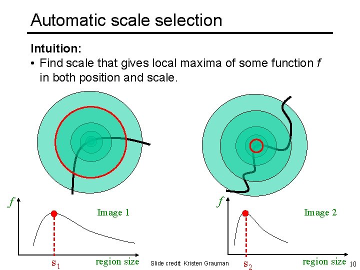
Automatic scale selection Intuition: • Find scale that gives local maxima of some function f in both position and scale. f Image 1 s 1 region size f Slide credit: Kristen Grauman Image 2 s 2 region size 10

What can be the “signature” function? 11 Slide credit: Kristen Grauman

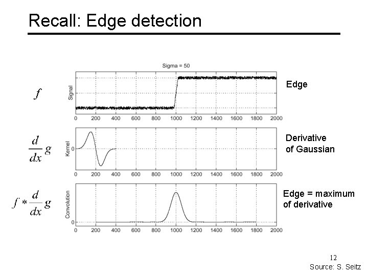
Recall: Edge detection f Edge Derivative of Gaussian Edge = maximum of derivative 12 Source: S. Seitz

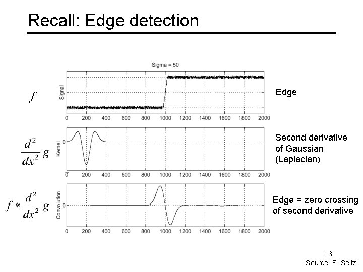
Recall: Edge detection f Edge Second derivative of Gaussian (Laplacian) Edge = zero crossing of second derivative 13 Source: S. Seitz

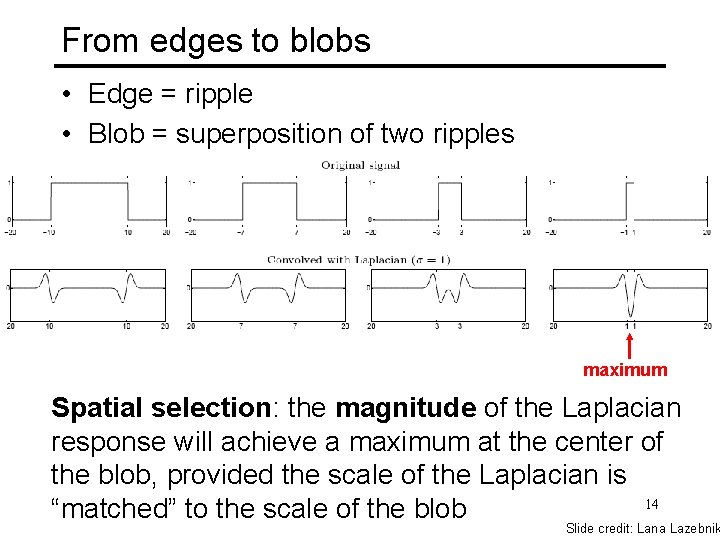
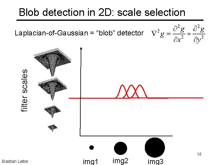
From edges to blobs • Edge = ripple • Blob = superposition of two ripples maximum Spatial selection: the magnitude of the Laplacian response will achieve a maximum at the center of the blob, provided the scale of the Laplacian is 14 “matched” to the scale of the blob Slide credit: Lana Lazebnik

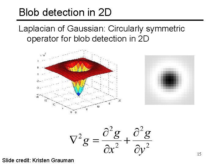
Blob detection in 2 D Laplacian of Gaussian: Circularly symmetric operator for blob detection in 2 D 15 Slide credit: Kristen Grauman

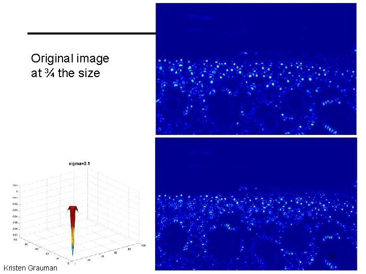
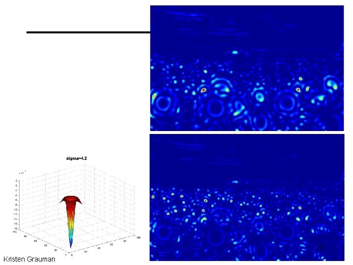
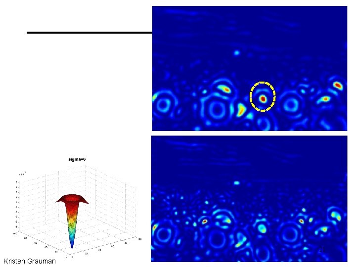
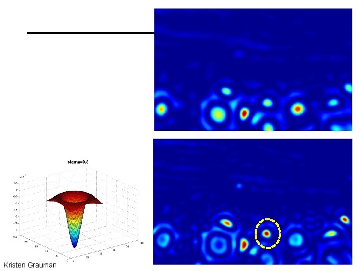
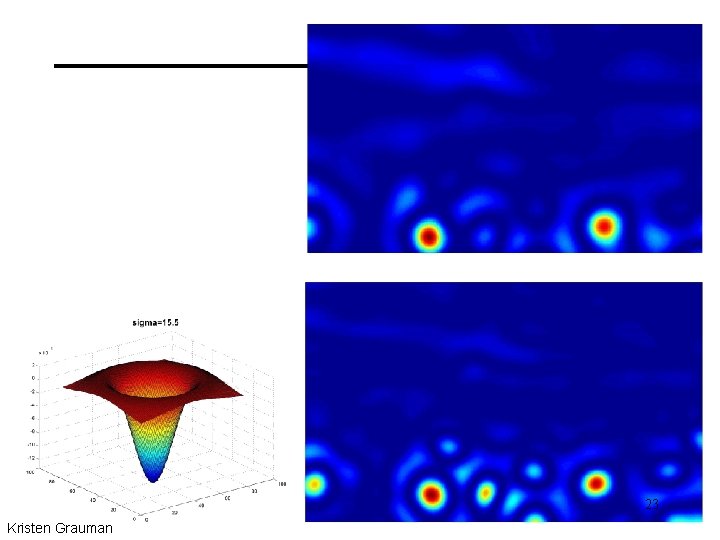
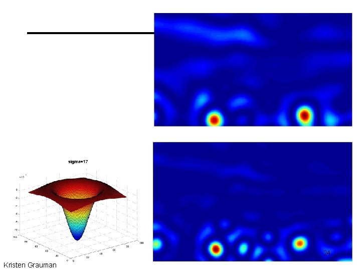
Blob detection in 2 D: scale selection filter scales Laplacian-of-Gaussian = “blob” detector Bastian Leibe img 1 img 2 16 img 3

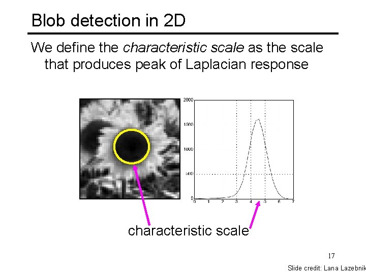
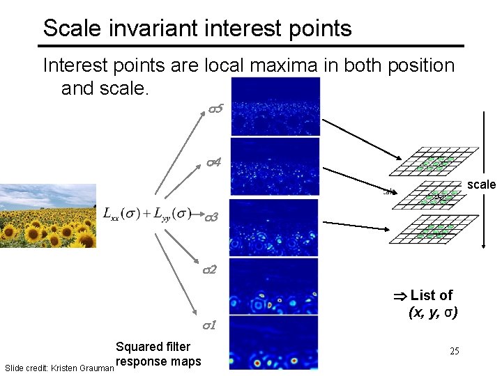
Blob detection in 2 D We define the characteristic scale as the scale that produces peak of Laplacian response characteristic scale 17 Slide credit: Lana Lazebnik

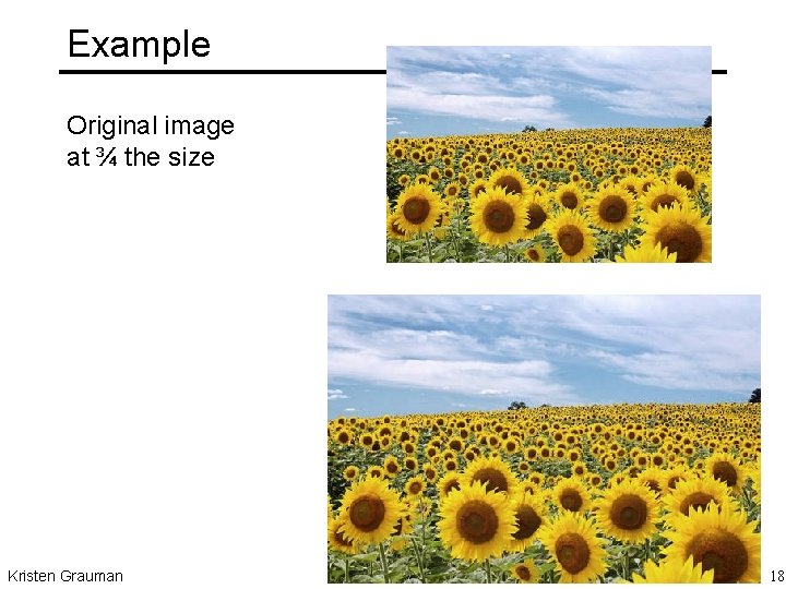
Example Original image at ¾ the size Kristen Grauman 18

Original image at ¾ the size 19 Kristen Grauman

20 Kristen Grauman

21 Kristen Grauman

22 Kristen Grauman

23 Kristen Grauman

24 Kristen Grauman

Scale invariant interest points Interest points are local maxima in both position and scale. s 5 s 4 scale s 3 s 2 s 1 Squared filter response maps Slide credit: Kristen Grauman List of (x, y, σ) 25

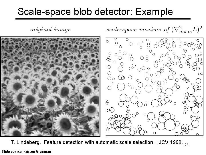
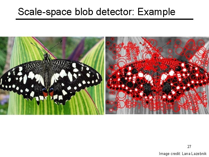
Scale-space blob detector: Example T. Lindeberg. Feature detection with automatic scale selection. IJCV 1998. Slide source: Kristen Grauman 26

Scale-space blob detector: Example 27 Image credit: Lana Lazebnik

Local features: main components 1) Detection: Identify the interest points 2) Description: Extract vector feature descriptor surrounding each interest point. 3) Matching: Determine correspondence between descriptors in two views 29 Slide credit: Kristen Grauman

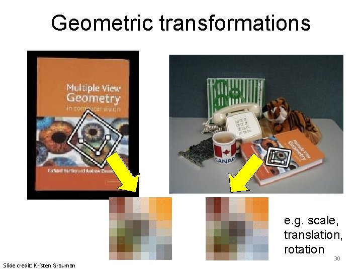
Geometric transformations e. g. scale, translation, rotation Slide credit: Kristen Grauman 30

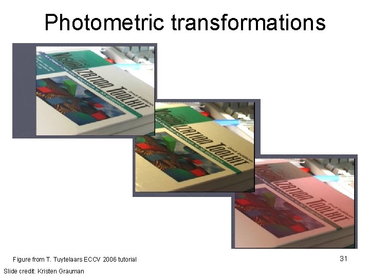
Photometric transformations Figure from T. Tuytelaars ECCV 2006 tutorial Slide credit: Kristen Grauman 31

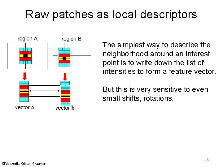
Raw patches as local descriptors The simplest way to describe the neighborhood around an interest point is to write down the list of intensities to form a feature vector. But this is very sensitive to even small shifts, rotations. Slide credit: Kristen Grauman 32

SIFT descriptor [Lowe 2004] • Use histograms to bin pixels within sub-patches according to their orientation. 0 Slide credit: Kristen Grauman 2 p Why subpatches? Why does SIFT have some illumination invariance? 33

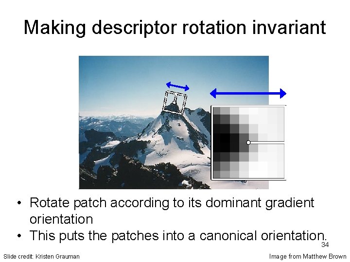
Making descriptor rotation invariant CSE 576: Computer Vision • Rotate patch according to its dominant gradient orientation • This puts the patches into a canonical orientation. 34 Slide credit: Kristen Grauman Image from Matthew Brown

SIFT descriptor [Lowe 2004] • Extraordinarily robust matching technique • Can handle changes in viewpoint • Up to about 60 degree out of plane rotation • Can handle significant changes in illumination • Sometimes even day vs. night (below) • • Fast and efficient—can run in real time Lots of code available • http: //people. csail. mit. edu/albert/ladypack/wiki/index. php/Known_implementations_of_SIFT 35 Steve Seitz

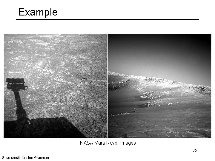
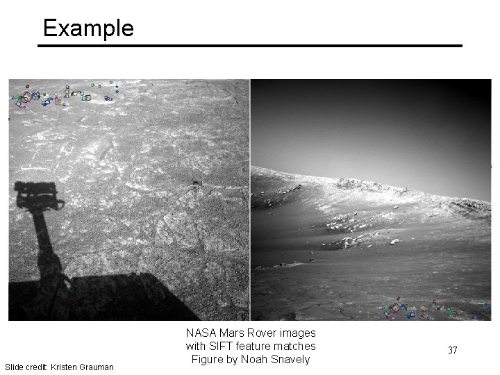
Example NASA Mars Rover images 36 Slide credit: Kristen Grauman

Example Slide credit: Kristen Grauman NASA Mars Rover images with SIFT feature matches Figure by Noah Snavely 37

SIFT properties • Invariant to – Scale – Rotation • Partially invariant to – Illumination changes – Camera viewpoint – Occlusion, clutter Slide credit: Kristen Grauman 38

Local features: main components 1) Detection: Identify the interest points 2) Description: Extract vector feature descriptor surrounding each interest point. 3) Matching: Determine correspondence between descriptors in two views 39 Slide credit: Kristen Grauman

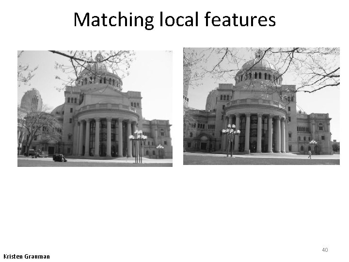
Matching local features Kristen Grauman 40

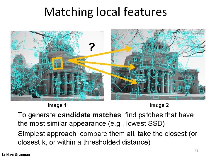
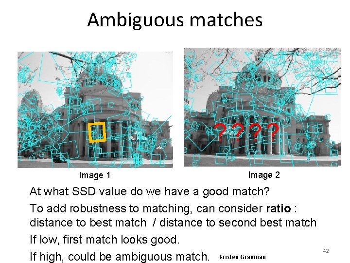
Matching local features ? Image 1 Image 2 To generate candidate matches, find patches that have the most similar appearance (e. g. , lowest SSD) Simplest approach: compare them all, take the closest (or closest k, or within a thresholded distance) Kristen Grauman 41

Ambiguous matches ? ? Image 1 Image 2 At what SSD value do we have a good match? To add robustness to matching, can consider ratio : distance to best match / distance to second best match If low, first match looks good. If high, could be ambiguous match. Kristen Grauman 42

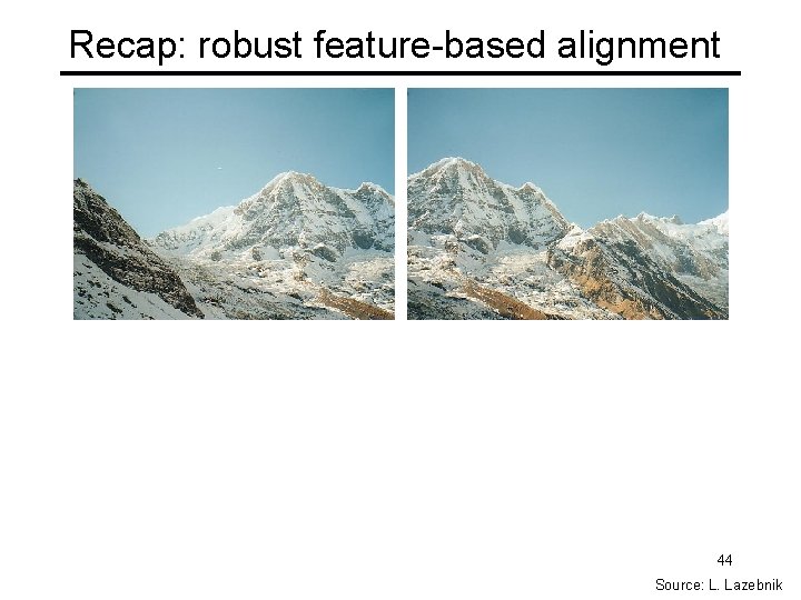
Recap: robust feature-based alignment 44 Source: L. Lazebnik

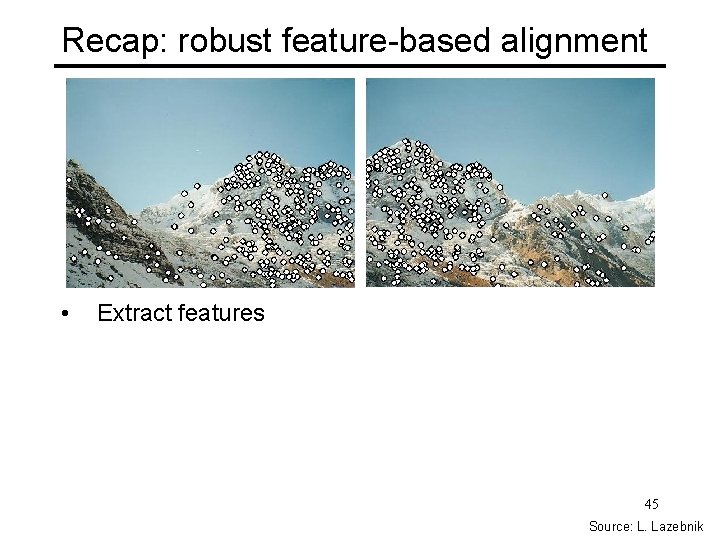
Recap: robust feature-based alignment • Extract features 45 Source: L. Lazebnik

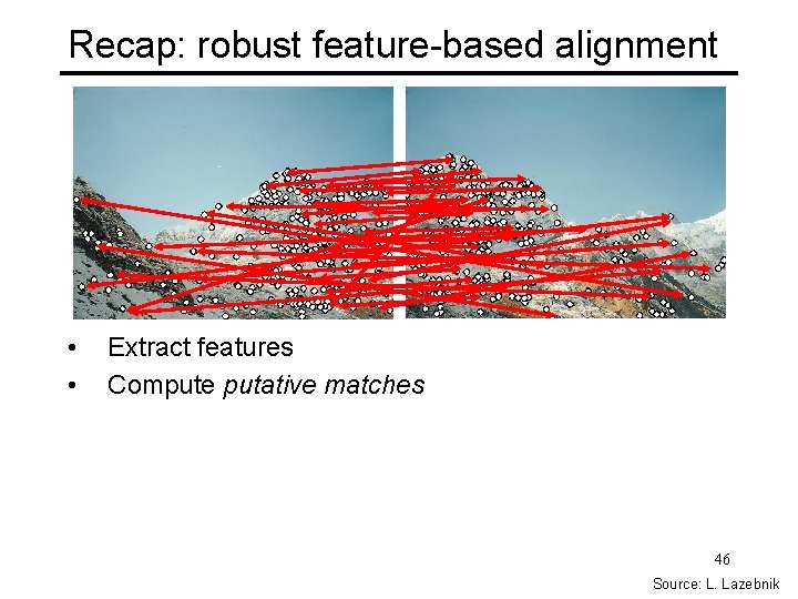
Recap: robust feature-based alignment • • Extract features Compute putative matches 46 Source: L. Lazebnik

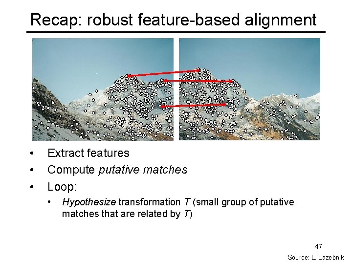
Recap: robust feature-based alignment • • • Extract features Compute putative matches Loop: • Hypothesize transformation T (small group of putative matches that are related by T) 47 Source: L. Lazebnik

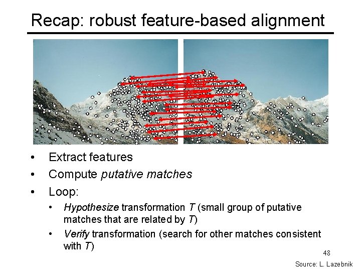
Recap: robust feature-based alignment • • • Extract features Compute putative matches Loop: • • Hypothesize transformation T (small group of putative matches that are related by T) Verify transformation (search for other matches consistent with T) 48 Source: L. Lazebnik

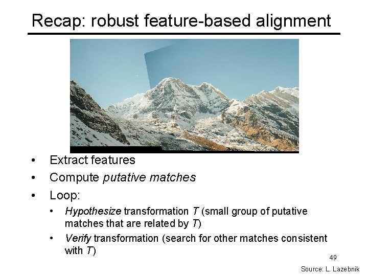
Recap: robust feature-based alignment • • • Extract features Compute putative matches Loop: • • Hypothesize transformation T (small group of putative matches that are related by T) Verify transformation (search for other matches consistent with T) 49 Source: L. Lazebnik

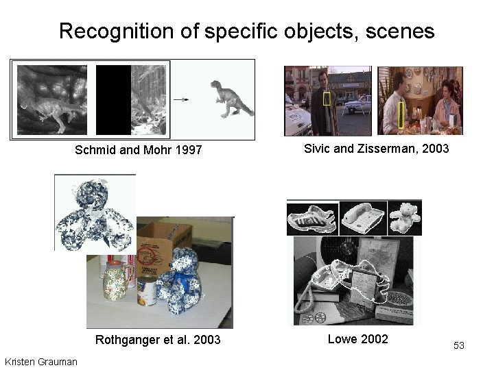
Applications of local invariant features • • Wide baseline stereo Motion tracking Panoramas Mobile robot navigation 3 D reconstruction Recognition … 50 Slide credit: Kristen Grauman

Wide baseline stereo [Image from T. Tuytelaars ECCV 2006 tutorial] Slide credit: Kristen Grauman 52

Recognition of specific objects, scenes Schmid and Mohr 1997 Rothganger et al. 2003 Kristen Grauman Sivic and Zisserman, 2003 Lowe 2002 53

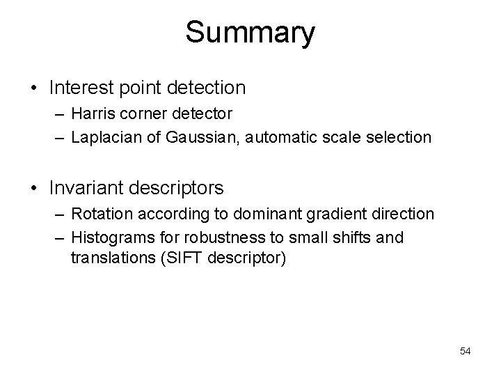
Summary • Interest point detection – Harris corner detector – Laplacian of Gaussian, automatic scale selection • Invariant descriptors – Rotation according to dominant gradient direction – Histograms for robustness to small shifts and translations (SIFT descriptor) 54

Questions? 55 Slide credit: Devi Parikh