CSE 202 Database Management Systems Lecture 8 Prepared

CSE 202 Database Management Systems Lecture #8 Prepared & Presented by Asst. Prof. Dr. Samsun M. BAŞARICI

Learning Objectives § Overview of some informal design guidelines for relation schemas § Understanding functional dependencies § Recognizing normal forms based on primary keys § Defining and differentiating second and third normal forms § Understanding Boyce-Codd normal form § Discriminating multivalued dependency and fourth normal form § Understanding join dependencies and fifth normal form § Applying relational database design algorithms 2

Outline § § § § Informal design guidelines for relation schemas Functional dependencies Normal forms based on primary keys General definitions of second and third normal forms Boyce-Codd normal form Multivalued dependency and fourth normal form Join dependencies and fifth normal form Relational database design algorithms 3

Part 1 Dependencies & Normal Forms 4

Introduction § Levels at which we can discuss goodness of relation schemas �Logical (or conceptual) level �Implementation (or physical storage) level § Approaches to database design: �Bottom-up or top-down 5

Informal Design Guidelines for Relation Schemas § Measures of quality �Making sure attribute semantics are clear �Reducing redundant information in tuples �Reducing NULL values in tuples �Disallowing possibility of generating spurious tuples 6

Imparting Clear Semantics to Attributes in Relations § Semantics of a relation �Meaning resulting from interpretation of attribute values in a tuple § Easier to explain semantics of relation �Indicates better schema design 7

Guideline 1 § Design relation schema so that it is easy to explain its meaning § Do not combine attributes from multiple entity types and relationship types into a single relation § Example of violating Guideline 1: Figure 15. 3 8

Guideline 1 (cont. ) 9

Redundant Information in Tuples and Update Anomalies § Grouping attributes into relation schemas �Significant effect on storage space § Storing natural joins of base relations leads to update anomalies § Types of update anomalies: �Insertion �Deletion �Modification 10

Guideline 2 § Design base relation schemas so that no update anomalies are present in the relations § If any anomalies are present: �Note them clearly �Make sure that the programs that update the database will operate correctly 11

NULL Values in Tuples § May group many attributes together into a “fat” relation �Can end up with many NULLs § Problems with NULLs �Wasted storage space �Problems understanding meaning 12

Guideline 3 § Avoid placing attributes in a base relation whose values may frequently be NULL § If NULLs are unavoidable: �Make sure that they apply in exceptional cases only, not to a majority of tuples 13

Generation of Spurious Tuples § Figure 15. 5(a) �Relation schemas EMP_LOCS and EMP_PROJ 1 § NATURAL JOIN �Result produces many more tuples than the original set of tuples in EMP_PROJ �Called spurious tuples �Represent spurious information that is not valid 14

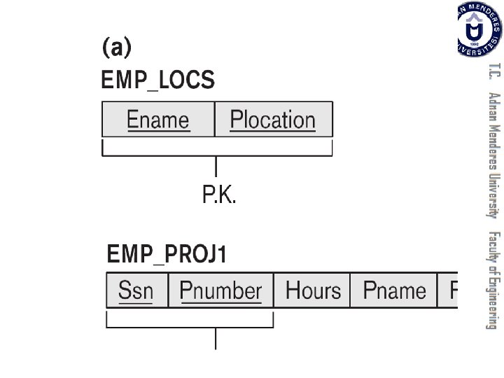
Guideline 4 § Design relation schemas to be joined with equality conditions on attributes that are appropriately related �Guarantees that no spurious tuples are generated § Avoid relations that contain matching attributes that are not (foreign key, primary key) combinations 16

Summary and Discussion of Design Guidelines § Anomalies cause redundant work to be done § Waste of storage space due to NULLs § Difficulty of performing operations and joins due to NULL values § Generation of invalid and spurious data during joins 17

Functional Dependencies § Formal tool for analysis of relational schemas § Enables us to detect and describe some of the abovementioned problems in precise terms § Theory of functional dependency 18

Definition of Functional Dependency § Constraint between two sets of attributes from the database § Property of semantics or meaning of the attributes § Legal relation states �Satisfy the functional dependency constraints 19

Definition of Functional Dependency (cont. ) § Given a populated relation �Cannot determine which FDs hold and which do not �Unless meaning of and relationships among attributes known �Can state that FD does not hold if there are tuples that show violation of such an FD 20

Normal Forms Based on Primary Keys § Normalization process § Approaches for relational schema design �Perform a conceptual schema design using a conceptual model then map conceptual design into a set of relations �Design relations based on external knowledge derived from existing implementation of files or forms or reports 21

Normalization of Relations § Takes a relation schema through a series of tests �Certify whether it satisfies a certain normal form �Proceeds in a top-down fashion § Normal form tests 22

Normalization of Relations (cont. ) § Properties that the relational schemas should have: �Nonadditive join property � Extremely critical �Dependency preservation property � Desirable but sometimes sacrificed for other factors 23

Practical Use of Normal Forms § Normalization carried out in practice �Resulting designs are of high quality and meet the desirable properties stated previously �Pays particular attention to normalization only up to 3 NF, BCNF, or at most 4 NF § Do not need to normalize to the highest possible normal form 24

Definitions of Keys and Attributes Participating in Keys § Definition of superkey and key § Candidate key �If more than one key in a relation schema � One is primary key � Others are secondary keys 25

First Normal Form § Part of the formal definition of a relation in the basic (flat) relational model § Only attribute values permitted are single atomic (or indivisible) values § Techniques to achieve first normal form �Remove attribute and place in separate relation �Expand the key �Use several atomic attributes 26

First Normal Form (cont. ) § Does not allow nested relations �Each tuple can have a relation within it § To change to 1 NF: �Remove nested relation attributes into a new relation �Propagate the primary key into it �Unnest relation into a set of 1 NF relations 27

28

Second Normal Form § Based on concept of full functional dependency �Versus partial dependency § Second normalize into a number of 2 NF relations �Nonprime attributes are associated only with part of primary key on which they are fully functionally dependent 29

Third Normal Form § Based on concept of transitive dependency § Problematic FD �Left-hand side is part of primary key �Left-hand side is a nonkey attribute 30

General Definitions of Second and Third Normal Forms 31

General Definitions of Second and Third Normal Forms (cont. ) § Prime attribute �Part of any candidate key will be considered as prime § Consider partial, full functional, and transitive dependencies with respect to all candidate keys of a relation 32

General Definition of Second Normal Form 33

34

General Definition of Third Normal Form 35

Boyce-Codd Normal Form § Every relation in BCNF is also in 3 NF �Relation in 3 NF is not necessarily in BCNF § Difference: �Condition which allows A to be prime is absent from BCNF § Most relation schemas that are in 3 NF are also in BCNF 36

37

Multivalued Dependency and Fourth Normal Form § Multivalued dependency (MVD) �Consequence of first normal form (1 NF) 38

Multivalued Dependency and Fourth Normal Form (cont. ) § Relations containing nontrivial MVDs �All-key relations § Fourth normal form (4 NF) �Violated when a relation has undesirable multivalued dependencies 39

Join Dependencies and Fifth Normal Form § Join dependency § Multiway decomposition into fifth normal form (5 NF) § Very peculiar semantic constraint �Normalization into 5 NF is very rarely done in practice 40

Join Dependencies and Fifth Normal Form (cont. ) 41

Part 2 Relational DB Design Algorithms 42

Designing a Set of Relations (1) § The Approach of Relational Synthesis (Bottom-up Design): �Assumes that all possible functional dependencies are known. �First constructs a minimal set of FDs �Then applies algorithms that construct a target set of 3 NF or BCNF relations. �Additional criteria may be needed to ensure the set of relations in a relational database are satisfactory. 43

Designing a Set of Relations (2) § Goals: �Lossless join property (a must) � Algorithm 16. 3 tests for general losslessness. �Dependency preservation property � Algorithm 16. 5 decomposes a relation into BCNF components by sacrificing the dependency preservation. �Additional normal forms � 4 NF (based on multi-valued dependencies) � 5 NF (based on join dependencies) 44

1. Properties of Relational Decompositions (1) § Relation Decomposition and Insufficiency of Normal Forms: �Universal Relation Schema: �A relation schema R = {A 1, A 2, …, An} that includes all the attributes of the database. �Universal relation assumption: �Every attribute name is unique. 45

Properties of Relational Decompositions (2) § Relation Decomposition and Insufficiency of Normal Forms (cont. ): �Decomposition: � The process of decomposing the universal relation schema R into a set of relation schemas D = {R 1, R 2, …, Rm} that will become the relational database schema by using the functional dependencies. �Attribute preservation condition: � Each attribute in R will appear in at least one relation schema Ri in the decomposition so that no attributes are “lost”. 46

Properties of Relational Decompositions (2) § Another goal of decomposition is to have each individual relation Ri in the decomposition D be in BCNF or 3 NF. § Additional properties of decomposition are needed to prevent from generating spurious tuples 47

Properties of Relational Decompositions (3) § Dependency Preservation Property of a Decomposition: �Definition: Given a set of dependencies F on R, the projection of F on Ri, denoted by p. Ri(F) where Ri is a subset of R, is the set of dependencies X Y in F+ such that the attributes in X υ Y are all contained in Ri. �Hence, the projection of F on each relation schema Ri in the decomposition D is the set of functional dependencies in F+, the closure of F, such that all their left- and right-hand-side attributes are in Ri. 48

Properties of Relational Decompositions (4) § Dependency Preservation Property of a Decomposition (cont. ): �Dependency Preservation Property: �A decomposition D = {R 1, R 2, . . . , Rm} of R is dependencypreserving with respect to F if the union of the projections of F on each Ri in D is equivalent to F; that is (( R 1(F)) υ. . . υ ( Rm(F)))+ = F+ � (See examples in Fig 15. 13 a and Fig 15. 12) § Claim 1: �It is always possible to find a dependency-preserving decomposition D with respect to F such that each relation Ri in D is in 3 nf. 49

Properties of Relational Decompositions (5) § Lossless (Non-additive) Join Property of a Decomposition: � Definition: Lossless join property: a decomposition D = {R 1, R 2, . . . , Rm} of R has the lossless (nonadditive) join property with respect to the set of dependencies F on R if, for every relation state r of R that satisfies F, the following holds, where * is the natural join of all the relations in D: * ( R 1(r), . . . , Rm(r)) = r � Note: The word loss in lossless refers to loss of information, not to loss of tuples. In fact, for “loss of information” a better term is “addition of spurious information” 50

Properties of Relational Decompositions (6) Lossless (Non-additive) Join Property of a Decomposition (cont. ): Algorithm 16. 3: Testing for Lossless Join Property � Input: A universal relation R, a decomposition D = {R 1, R 2, . . . , Rm} of R, and a set F of functional dependencies. 1. Create an initial matrix S with one row i for each relation Ri in D, and one column j for each attribute Aj in R. 2. Set S(i, j): =bij for all matrix entries. (* each bij is a distinct symbol associated with indices (i, j) *). 3. For each row i representing relation schema Ri {for each column j representing attribute Aj {if (relation Ri includes attribute Aj) then set S(i, j): = aj; }; }; � (* each aj is a distinct symbol associated with index (j) *) § § 51

Properties of Relational Decompositions (7) § Lossless (Non-additive) Join Property of a Decomposition (cont. ): § Algorithm 16. 3: Testing for Lossless Join Property 4. Repeat the following loop until a complete loop execution results in no changes to S {for each functional dependency X Y in F {for all rows in S which have the same symbols in the columns corresponding to attributes in X {make the symbols in each column that correspond to an attribute in Y be the same in all these rows as follows: If any of the rows has an “a” symbol for the column, set the other rows to that same “a” symbol in the column. If no “a” symbol exists for the attribute in any of the rows, choose one of the “b” symbols that appear in one of the rows for the attribute and set the other rows to that same “b” symbol in the column ; }; }; }; 5. If a row is made up entirely of “a” symbols, then the decomposition has the lossless join property; otherwise it does not. 52

Properties of Relational Decompositions (8) Lossless (nonadditive) join test for n-ary decompositions. (a) Case 1: Decomposition of EMP_PROJ into EMP_PROJ 1 and EMP_LOCS fails test. (b) A decomposition of EMP_PROJ that has the lossless join property. 53

Properties of Relational Decompositions (9) Lossless (nonadditive) join test for n-ary decompositions. (c) Case 2: Decomposition of EMP_PROJ into EMP, PROJECT, and WORKS_ON satisfies test. 54

Properties of Relational Decompositions (10) § Testing Binary Decompositions for Lossless Join Property �Binary Decomposition: Decomposition of a relation R into two relations. �PROPERTY LJ 1 (lossless join test for binary decompositions): A decomposition D = {R 1, R 2} of R has the lossless join property with respect to a set of functional dependencies F on R if and only if either f. d. ((R 1 ∩ R 2) (R 1 - R 2)) is in F+, or � The f. d. ((R 1 ∩ R 2) (R 2 - R 1)) is in F+. � The 55

Properties of Relational Decompositions (11) § Successive Lossless Join Decomposition: �Claim 2 (Preservation of non-additivity in successive decompositions): � If a decomposition D = {R 1, R 2, . . . , Rm} of R has the lossless (non-additive) join property with respect to a set of functional dependencies F on R, � and if a decomposition Di = {Q 1, Q 2, . . . , Qk} of Ri has the lossless (non-additive) join property with respect to the projection of F on Ri, � then the decomposition D 2 = {R 1, R 2, . . . , Ri-1, Q 2, . . . , Qk, Ri+1, . . . , Rm} of R has the non-additive join property with respect to F. 56

2. Algorithms for Relational Database Schema Design (1) § Algorithm 16. 4: Relational Synthesis into 3 NF with Dependency Preservation (Relational Synthesis Algorithm) � Input: A universal relation R and a set of functional dependencies F on the attributes of R. 1. Find a minimal cover G for F (use Algorithm 16. 2); 2. For each left-hand-side X of a functional dependency that appears in G, create a relation schema in D with attributes {X υ {A 1} υ {A 2}. . . υ {Ak}}, where X A 1, X A 2, . . . , X Ak are the only dependencies in G with X as left-hand-side (X is the key of this relation) ; 3. Place any remaining attributes (that have not been placed in any relation) in a single relation schema to ensure the attribute preservation property. � Claim 3: Every relation schema created by Algorithm 16. 4 is in 3 NF. 57

Algorithms for Relational Database Schema Design (2) § Algorithm 16. 5: Relational Decomposition into BCNF with Lossless (non-additive) join property � Input: A universal relation R and a set of functional dependencies F on the attributes of R. 1. Set D : = {R}; 2. While there is a relation schema Q in D that is not in BCNF do { choose a relation schema Q in D that is not in BCNF; find a functional dependency X Y in Q that violates BCNF; replace Q in D by two relation schemas (Q - Y) and (X υ Y); }; Assumption: No null values are allowed for the join attributes. 58

Algorithms for Relational Database Schema Design (3) § Algorithm 16. 6 Relational Synthesis into 3 NF with Dependency Preservation and Lossless (Non-Additive) Join Property � Input: A universal relation R and a set of functional dependencies F on the attributes of R. 1. Find a minimal cover G for F (Use Algorithm 16. 2). 2. For each left-hand-side X of a functional dependency that appears in G, create a relation schema in D with attributes {X υ {A 1} υ {A 2}. . . υ {Ak}}, where X A 1, X A 2, . . . , X –>Ak are the only dependencies in G with X as left-hand-side (X is the key of this relation). 3. If none of the relation schemas in D contains a key of R, then create one more relation schema in D that contains attributes that form a key of R. (Use Algorithm 16. 4 a to find the key of R) 59

Algorithms for Relational Database Schema Design (4) § Algorithm 16. 2 a Finding a Key K for R Given a set F of Functional Dependencies �Input: A universal relation R and a set of functional dependencies F on the attributes of R. 1. Set K : = R; 2. For each attribute A in K { Compute (K - A)+ with respect to F; If (K - A)+ contains all the attributes in R, then set K : = K - {A}; } 60

Algorithms for Relational Database Schema Design (5) 61

Algorithms for Relational Database Schema Design (5) 62

Algorithms for Relational Database Schema Design (6) 63

Algorithms for Relational Database Schema Design (7) 64

Algorithms for Relational Database Schema Design (8) § Discussion of Normalization Algorithms: § Problems: �The database designer must first specify all the relevant functional dependencies among the database attributes. �These algorithms are not deterministic in general. �It is not always possible to find a decomposition into relation schemas that preserves dependencies and allows each relation schema in the decomposition to be in BCNF (instead of 3 NF as in Algorithm 16. 6). 65

Algorithms for Relational Database Schema Design (9) 66

3. Multivalued Dependencies and Fourth Normal Form (1) (a) The EMP relation with two MVDs: ENAME —>> PNAME and ENAME —>> DNAME. (b) Decomposing the EMP relation into two 4 NF relations EMP_PROJECTS and EMP_DEPENDENTS. 67

3. Multivalued Dependencies and Fourth Normal Form (2) (c) The relation SUPPLY with no MVDs is in 4 NF but not in 5 NF if it has the JD(R 1, R 2, R 3). (d) Decomposing the relation SUPPLY into the 5 NF relations R 1, R 2, and R 3. 68

Multivalued Dependencies and Fourth Normal Form (3) Definition: § A multivalued dependency (MVD) X —>> Y specified on relation schema R, where X and Y are both subsets of R, specifies the following constraint on any relation state r of R: If two tuples t 1 and t 2 exist in r such that t 1[X] = t 2[X], then two tuples t 3 and t 4 should also exist in r with the following properties, where we use Z to denote (R 2 (X υ Y)): � t 3[X] = t 4[X] = t 1[X] = t 2[X]. � t 3[Y] = t 1[Y] and t 4[Y] = t 2[Y]. t 3[Z] = t 2[Z] and t 4[Z] = t 1[Z]. An MVD X —>> Y in R is called a trivial MVD if (a) Y is a subset of X, or (b) X υ Y = R. � § 69

Multivalued Dependencies and Fourth Normal Form (4) § Inference Rules for Functional and Multivalued Dependencies: � � � IR 1 (reflexive rule for FDs): If X Y, then X –> Y. IR 2 (augmentation rule for FDs): {X –> Y} XZ –> YZ. IR 3 (transitive rule for FDs): {X –> Y, Y –>Z} X –> Z. IR 4 (complementation rule for MVDs): {X —>> Y} X —>> (R – (X Y))}. IR 5 (augmentation rule for MVDs): If X —>> Y and W Z then WX —>> YZ. IR 6 (transitive rule for MVDs): {X —>> Y, Y —>> Z} X —>> (Z 2 Y). IR 7 (replication rule for FD to MVD): {X –> Y} X —>> Y. � IR 8 (coalescence rule for FDs and MVDs): If X —>> Y and there exists W with the properties that � (a) W Y is empty, (b) W –> Z, and (c) Y Z, then X –> Z. � 70

Multivalued Dependencies and Fourth Normal Form (5) Definition: § A relation schema R is in 4 NF with respect to a set of dependencies F (that includes functional dependencies and multivalued dependencies) if, for every nontrivial multivalued dependency X —>> Y in F+, X is a superkey for R. � Note: F+ is the (complete) set of all dependencies (functional or multivalued) that will hold in every relation state r of R that satisfies F. It is also called the closure of F. 71

Multivalued Dependencies and Fourth Normal Form (6) 72

Multivalued Dependencies and Fourth Normal Form (7) Lossless (Non-additive) Join Decomposition into 4 NF Relations: § PROPERTY LJ 1’ � The relation schemas R 1 and R 2 form a lossless (nonadditive) join decomposition of R with respect to a set F of functional and multivalued dependencies if and only if � � (R 1 ∩ R 2) —>> (R 1 - R 2) or by symmetry, if and only if � (R 1 ∩ R 2) —>> (R 2 - R 1)). 73

Multivalued Dependencies and Fourth Normal Form (8) Algorithm 16. 7: Relational decomposition into 4 NF relations with non-additive join property § Input: A universal relation R and a set of functional and multivalued dependencies F. 1. 2. Set D : = { R }; While there is a relation schema Q in D that is not in 4 NF do { choose a relation schema Q in D that is not in 4 NF; find a nontrivial MVD X —>> Y in Q that violates 4 NF; replace Q in D by two relation schemas (Q - Y) and (X υ Y); }; 74

4. Join Dependencies and Fifth Normal Form (1) Definition: § A join dependency (JD), denoted by JD(R 1, R 2, . . . , Rn), specified on relation schema R, specifies a constraint on the states r of R. � � § The constraint states that every legal state r of R should have a non-additive join decomposition into R 1, R 2, . . . , Rn; that is, for every such r we have * ( R 1(r), R 2(r), . . . , Rn(r)) = r Note: an MVD is a special case of a JD where n = 2. A join dependency JD(R 1, R 2, . . . , Rn), specified on relation schema R, is a trivial JD if one of the relation schemas Ri in JD(R 1, R 2, . . . , Rn) is equal to R. 75

Join Dependencies and Fifth Normal Form (2) Definition: § A relation schema R is in fifth normal form (5 NF) (or Project-Join Normal Form (PJNF)) with respect to a set F of functional, multivalued, and join dependencies if, � for every nontrivial join dependency JD(R 1, R 2, . . . , Rn) in F+ (that is, implied by F), � every Ri is a superkey of R. 76

Relation SUPPLY with Join Dependency and Conversion to Fifth Normal Form 77

5. Inclusion Dependencies (1) Definition: § An inclusion dependency R. X < S. Y between two sets of attributes—X of relation schema R, and Y of relation schema S —specifies the constraint that, at any specific time when r is a relation state of R and s a relation state of S, we must have § Note: � � � X(r(R)) Y(s(S)) The ? (subset) relationship does not necessarily have to be a proper subset. The sets of attributes on which the inclusion dependency is specified—X of R and Y of S—must have the same number of attributes. In addition, the domains for each pair of corresponding attributes should be compatible. 78

Inclusion Dependencies (2) § Objective of Inclusion Dependencies: � § To formalize two types of interrelational constraints which cannot be expressed using F. D. s or MVDs: � Referential integrity constraints � Class/subclass relationships Inclusion dependency inference rules � � IDIR 1 (reflexivity): R. X < R. X. IDIR 2 (attribute correspondence): If R. X < S. Y � � � where X = {A 1, A 2 , . . . , An} and Y = B 2, . . . , Bn} and Ai Corresponds-to Bi, then R. Ai < S. Bi for 1 ≤ i ≤ n. {B 1, IDIR 3 (transitivity): If R. X < S. Y and S. Y < T. Z, then R. X < T. Z. 79

6. Other Dependencies and Normal Forms (1) Template Dependencies: § § Template dependencies provide a technique for representing constraints in relations that typically have no easy and formal definitions. The idea is to specify a template—or example—that defines each constraint or dependency. There are two types of templates: � tuple-generating templates � constraint-generating templates. A template consists of a number of hypothesis tuples that are meant to show an example of the tuples that may appear in one or more relations. The other part of the template is the template conclusion. 80

Other Dependencies and Normal Forms (2) 81

Other Dependencies and Normal Forms (3) 82

Other Dependencies and Normal Forms (4) Domain-Key Normal Form (DKNF): § § Definition: � A relation schema is said to be in DKNF if all constraints and dependencies that should hold on the valid relation states can be enforced simply by enforcing the domain constraints and key constraints on the relation. The idea is to specify (theoretically, at least) the “ultimate normal form” that takes into account all possible types of dependencies and constraints. . For a relation in DKNF, it becomes very straightforward to enforce all database constraints by simply checking that each attribute value in a tuple is of the appropriate domain and that every key constraint is enforced. The practical utility of DKNF is limited 83

Additional Material (Again) Logical DB Design 84

Chapter 7 Logical Database Design Fundamentals of Database Management Systems, 2 nd ed. by Mark L. Gillenson, Ph. D. University of Memphis John Wiley & Sons, Inc.

Chapter Objectives ¨ Describe the concept of logical database design. ¨ Design relational databases by converting entity-relationship diagrams into relational tables. ¨ Describe the data normalization process. 7 -86

Chapter Objectives ¨ Perform the data normalization process. ¨ Test tables for irregularities using the data normalization process. 7 -87

Logical Database Design ¨ The process of deciding how to arrange the attributes of the entities in the business environment into database structures, such as the tables of a relational database. ¨ The goal is to create well structured tables that properly reflect the company’s business environment. 7 -88

Logical Design of Relational Database Systems ¨ (1) The conversion of E-R diagrams into relational tables. ¨ (2) The data normalization technique. ¨ (3) The use of the data normalization technique to test the tables resulting from the E-R diagram conversions. 7 -89

Converting E-R Diagrams into Relational Tables ¨ Each entity will convert to a table. ¨ Each many-to-many relationship or associative entity will convert to a table. ¨ During the conversion, certain rules must be followed to ensure that foreign keys appear in their proper places in the tables. 7 -90

Converting a Simple Entity ¨ The table simply contains the attributes that were specified in the entity box. ¨ Salesperson Number is underlined to indicate that it is the unique identifier of the entity and the primary key of the table. 7 -91

Converting Entities in Binary Relationships: One-to-One ¨ There are three options for designing tables to represent this data. 7 -92

One-to-One: Option #1 ¨ The two entities are combined into one relational table. 7 -93

One-to-One: Option #2 ¨ Separate tables for the SALESPERSON and OFFICE entities, with Office Number as a foreign key in the SALESPERSON table. 7 -94

One-to-One: Option #3 ¨ Separate tables for the SALESPERSON and OFFICE entities, with Salesperson Number as a foreign key in the OFFICE table. 7 -95

Converting Entities in Binary Relationships: One-to-Many ¨ The unique identifier of the entity on the “one side” of the one-to-many relationship is placed as a foreign key in the table representing the entity on the “many side. ” ¨ So, the Salesperson Number attribute is placed in the CUSTOMER table as a foreign key. 7 -96

Converting Entities in Binary Relationships: One-to-Many 7 -97

Converting Entities in Binary Relationships: Many-to-Many ¨ E-R diagram with the many-to-many binary relationship and the equivalent diagram using an associative entity. 7 -98

Converting Entities in Binary Relationships: Many-to-Many ¨ An E-R diagram with two entities in a many-tomany relationship converts to three relational tables. ¨ Each of the two entities converts to a table with its own attributes but with no foreign keys (regarding this relationship). ¨ In addition, there must be a third “many-to-many” table for the many-to-many relationship. 7 -99

Converting Entities in Binary Relationships: Many-to-Many ¨ The primary key of SALE is the combination of the unique identifiers of the two entities in the manyto-many relationship. Additional attributes are the intersection data. 7 -100

Converting Entities in Unary Relationships: One-to-One ¨ With only one entity type involved and with a one-toone relationship, the conversion requires only one table. 7 -101

Converting Entities in Unary Relationships: One-to-Many ¨ Very similar to the oneto-one unary case. 7 -102

Converting Entities in Unary Relationships: Many-to-Many ¨ This relationship requires two tables in the conversion. ¨ The PRODUCT table has no foreign keys. 7 -103

Converting Entities in Unary Relationships: Many-to-Many ¨ A second table is created since in the conversion of a many-to-many relationship of any degree — unary, binary, or ternary — the number of tables will be equal to the number of entity types (one, two, or three, respectively) plus one more table for the many-to-many relationship. 7 -104

Converting Entities in Ternary Relationships ¨ The primary key of the SALE table is the combination of the unique identifiers of the three entities involved, plus the Date attribute. 7 -105

Designing the General Hardware Company Database 7 -106

Designing the Good Reading Bookstores Database 7 -107

Designing the World Music Association Database 7 -108

Designing the Lucky Rent-A-Car Database 7 -109

The Data Normalization Process ¨ A methodology for organizing attributes into tables so that redundancy among the nonkey attributes is eliminated. ¨ The output of the data normalization process is a properly structured relational database. 7 -110

The Data Normalization Technique ¨ Input: ª all the attributes that must be incorporated into the database ª a list of all the defining associations between the attributes (i. e. , the functional dependencies). • a means of expressing that the value of one particular attribute is associated with a single, specific value of another attribute. • If we know that one of these attributes has a particular value, then the other attribute must have some other value. 7 -111

Functional Dependence Salesperson Number Salesperson Name ¨ Salesperson Number is the determinant. ¨ The value of Salesperson Number determines the value of Salesperson Name. ¨ Salesperson Name is functionally dependent on Salesperson Number. 7 -112

General Hardware Environment: SALESPERSON and PRODUCT 7 -113

Steps in the Data Normalization Process ¨ First Normal Form ¨ Second Normal Form ¨ Third Normal Form 7 -114

The Data Normalization Process ¨ Once the attributes are arranged in third normal form, the group of tables that they comprise is a well-structured relational database with no data redundancy. ¨ A group of tables is said to be in a particular normal form if every table in the group is in that normal form. ¨ The data normalization process is progressive. ª For example, if a group of tables is in second normal form, it is also in first normal form. 7 -115

General Hardware Company: Unnormalized Data ¨ Records contain multivalued attributes. 7 -116

General Hardware Company: First Normal Form ¨ The attributes under consideration have been listed in one table, and a primary key has been established. ¨ The number of records has been increased so that every attribute of every record has just one value. ¨ The multivalued attributes have been eliminated. 7 -117

General Hardware Company: First Normal Form 7 -118

General Hardware Company: First Normal Form ¨ First normal form is merely a starting point in the normalization process. ¨ First normal form contains a great deal of data redundancy. ª Three records involve salesperson 137, so there are three places in which his name is listed as Baker, his commission percentage is listed as 10, and so on. ª Two records involve product 19440 and this product’s name is listed twice as Hammer and its unit price is listed twice as 17. 50. 7 -119

General Hardware Company: Second Normal Form ¨ No Partial Functional Dependencies ª Every nonkey attribute must be fully functionally dependent on the entire key of that table. ª A nonkey attribute cannot depend on only part of the key. 7 -120

General Hardware Company: Second Normal Form ¨ In SALESPERSON, Salesperson Number is the sole primary key attribute. Every nonkey attribute of the table is fully defined just by Salesperson Number. ¨ Similar logic for PRODUCT and QUANTITY tables. 7 -121

General Hardware Company: Second Normal Form 7 -122

General Hardware Company: Third Normal Form ¨ Does not allow transitive dependencies in which one nonkey attribute is functionally dependent on another. ¨ Nonkey attributes are not allowed to define other nonkey attributes. 7 -123

General Hardware Company: Third Normal Form 7 -124

General Hardware Company: Third Normal Form 7 -125

General Hardware Company: Third Normal Form ¨ Important points about the third normal form structure are: ª It is completely free of data redundancy. ª All foreign keys appear where needed to logically tie together related tables. ª It is the same structure that would have been derived from a properly drawn entity-relationship diagram of the same business environment. 7 -126

Candidate Keys as Determinants ¨ There is one exception to the rule that in third normal form, nonkey attributes are not allowed to define other nonkey attributes. ¨ The rule does not hold if the defining nonkey attribute is a candidate key of the table. ¨ Candidate keys in a relation may define other nonkey attributes without violating third normal form. 7 -127

General Hardware Company: Functional Dependencies 7 -128

General Hardware Company: First Normal Form 7 -129

Good Reading Bookstores: Functional Dependencies 7 -130

World Music Association: Functional Dependencies 7 -131

Lucky Rent-A-Car: Functional Dependencies 7 -132

Data Normalization Check ¨ The basic idea in checking the structural worthiness of relational tables, created through E-R diagram conversion, with the data normalization rules is to: ª Check to see if there any partial functional dependencies. ª Check to see if there any transitive dependencies. 7 -133

Creating a Table with SQL CREATE TABLE SALESPERSON (SPNUM CHAR(3) PRIMARY KEY, SPNAME CHAR(12) COMMPERCT DECIMAL(3, 0) YEARHIRE CHAR(4) OFFNUM CHAR(3) ); Dropping a Table with SQL DROP TABLE SALESPERSON; 7 -134

Creating a View with SQL CREATE VIEW EMPLOYEE AS SELECT SPNUM, SPNAME, YEARHIRE FROM SLAESPERSON; Dropping a View with SQL DROP VIEW EMPLOYEE ; 7 -135

The SQL Update, Insert, and Delete Commands UPDATE SALESPERSON SET COMMPERCT = 12 WHERE SPNUM = ‘ 204’; INSERT INTO SALESPERSON VALUES (‘ 489’, ‘Quinlan’, 15, ‘ 2011’, ‘ 59’); DELETE FROM SALESPERSON WHERE SPNUM = ‘ 186’; 7 -136

Next Lecture Physical DB Design, Files, Hashes, Indexing 137

References § Ramez Elmasri, Shamkant Navathe; “Fundamentals of Database Systems”, 6 th Ed. , Pearson, 2014 § Mark L. Gillenson; “Fundamentals of Database Management Systems”, 2 nd Ed. , John Wiley, 2012 § Universität Hamburg, Fachbereich Informatik, Einführung in Datenbanksysteme, Lecture Notes, 1999 138