KLMH VLSI Physical Design From Graph Partitioning to

© KLMH VLSI Physical Design: From Graph Partitioning to Timing Closure Chapter 6 – Detailed Routing Original Authors: 1 Lienig Andrew B. Kahng, Jens Lienig, Igor L. Markov, Jin Hu

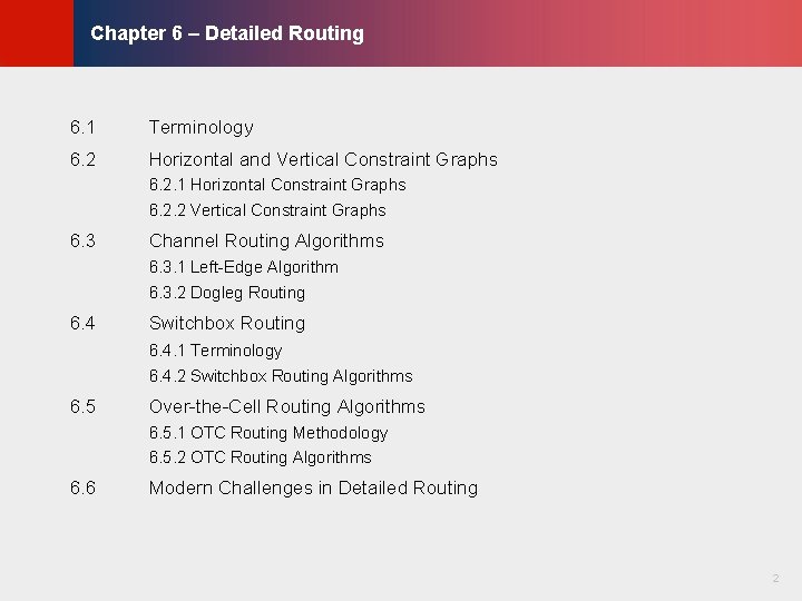
© KLMH Chapter 6 – Detailed Routing 6. 1 Terminology 6. 2 Horizontal and Vertical Constraint Graphs 6. 2. 1 Horizontal Constraint Graphs 6. 2. 2 Vertical Constraint Graphs 6. 3 Channel Routing Algorithms 6. 3. 1 Left-Edge Algorithm 6. 3. 2 Dogleg Routing 6. 4 Switchbox Routing 6. 4. 1 Terminology 6. 4. 2 Switchbox Routing Algorithms 6. 5 Over-the-Cell Routing Algorithms 6. 5. 1 OTC Routing Methodology 6. 5. 2 OTC Routing Algorithms Modern Challenges in Detailed Routing 2 Lienig 6. 6

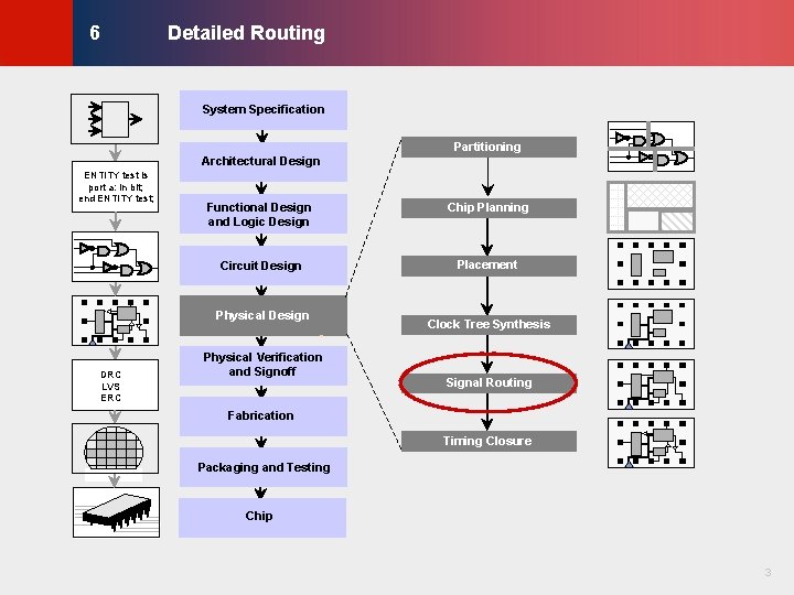
Detailed Routing © KLMH 6 System Specification Partitioning Architectural Design Functional Design and Logic Design Chip Planning Circuit Design Placement Physical Design DRC LVS ERC Physical Verification and Signoff Clock Tree Synthesis Signal Routing Fabrication Timing Closure Packaging and Testing Chip 3 Lienig ENTITY test is port a: in bit; end ENTITY test;

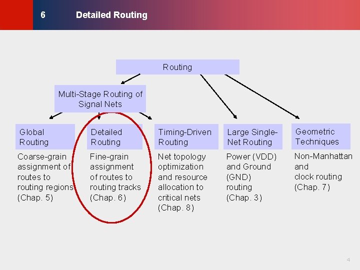
Detailed Routing © KLMH 6 Routing Global Routing Detailed Routing Timing-Driven Routing Large Single. Net Routing Geometric Techniques Coarse-grain assignment of routes to routing regions (Chap. 5) Fine-grain assignment of routes to routing tracks (Chap. 6) Net topology optimization and resource allocation to critical nets (Chap. 8) Power (VDD) and Ground (GND) routing (Chap. 3) Non-Manhattan and clock routing (Chap. 7) 4 Lienig Multi-Stage Routing of Signal Nets

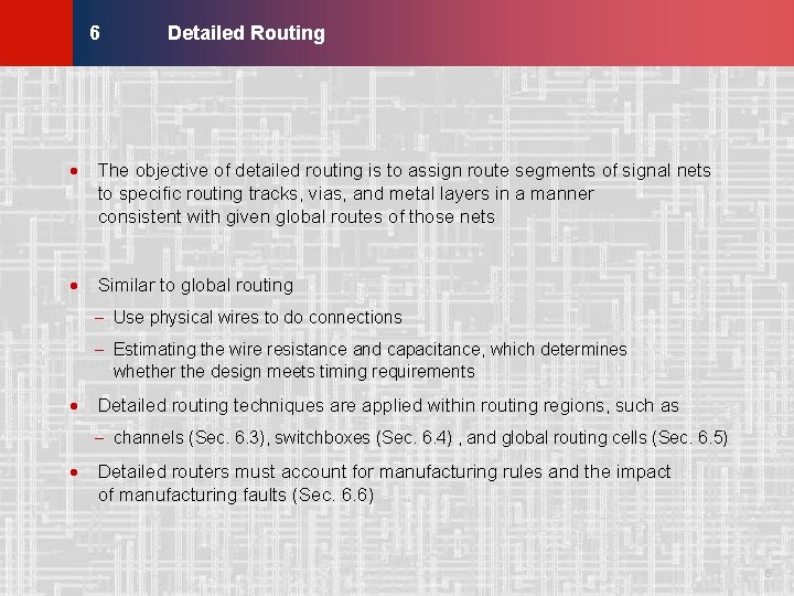
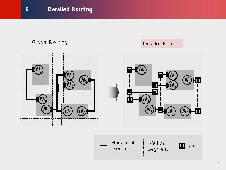
Detailed Routing © KLMH 6 · The objective of detailed routing is to assign route segments of signal nets to specific routing tracks, vias, and metal layers in a manner consistent with given global routes of those nets · Similar to global routing - Use physical wires to do connections - Estimating the wire resistance and capacitance, which determines whether the design meets timing requirements · Detailed routing techniques are applied within routing regions, such as - channels (Sec. 6. 3), switchboxes (Sec. 6. 4) , and global routing cells (Sec. 6. 5) 5 Lienig · Detailed routers must account for manufacturing rules and the impact of manufacturing faults (Sec. 6. 6)

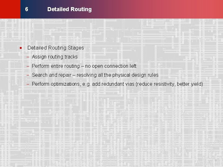
Detailed Routing © KLMH 6 · Detailed Routing Stages - Assign routing tracks - Perform entire routing – no open connection left - Search and repair – resolving all the physical design rules 6 Lienig - Perform optimizations, e. g. add redundant vias (reduce resistivity, better yield)

Detailed Routing © KLMH 6 Global Routing N 1 N 3 N 3 N 1 N 2 Horizontal Segment Vertical Segment N 1 N 2 Via 7 Lienig N 3 Detailed Routing

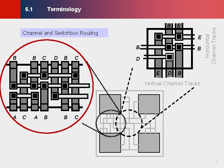
B E Channel and Switchbox Routing E B B B C D B C © KLMH Terminology B D E D Horizontal Channel Tracks 6. 1 B Vertical Channel Tracks C A B B C 8 Lienig A

Terminology © KLMH 6. 1 Channel Routing Standard Cell Row Power Rail Channel 9 Lienig External Pad

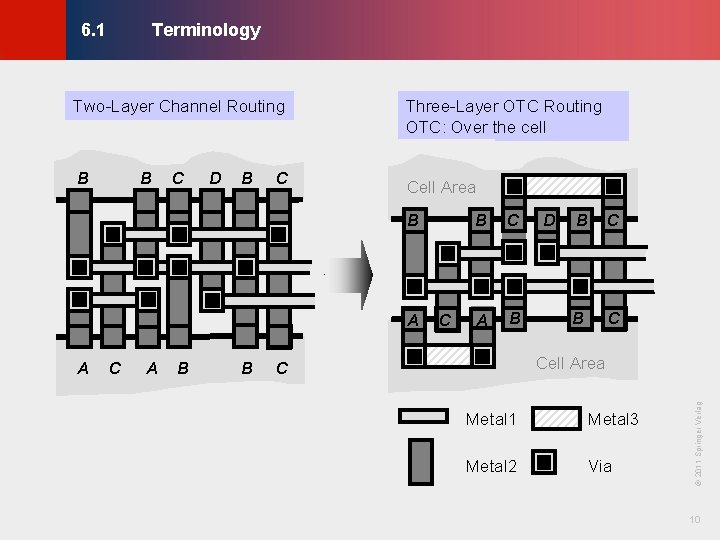
Terminology © KLMH 6. 1 B C D B C Cell Area B A A C A B B C A B D B C Cell Area C Metal 1 Metal 3 Metal 2 Via © 2011 Springer Verlag B Three-Layer OTC Routing OTC: Over the cell 10 Lienig Two-Layer Channel Routing

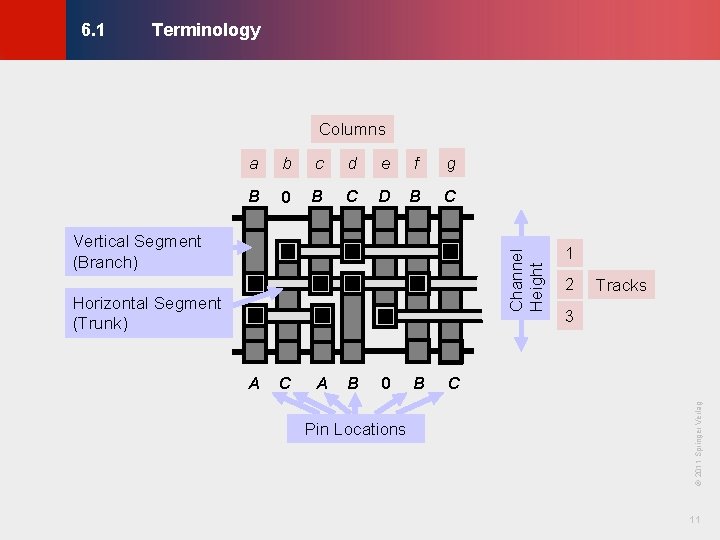
Terminology © KLMH 6. 1 Columns a b c d e f g B 0 B C D B C Channel Height Vertical Segment (Branch) Horizontal Segment (Trunk) A B 0 Pin Locations B Tracks 3 C © 2011 Springer Verlag C 2 11 Lienig A 1

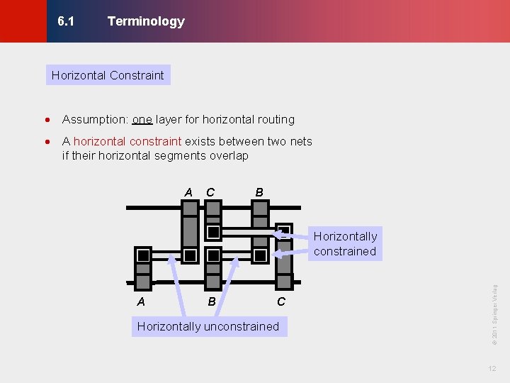
Terminology © KLMH 6. 1 Horizontal Constraint · Assumption: one layer for horizontal routing · A horizontal constraint exists between two nets if their horizontal segments overlap A C B B C Horizontally unconstrained 12 Lienig A © 2011 Springer Verlag Horizontally constrained

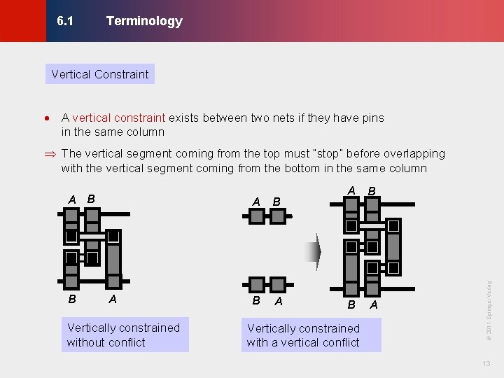
Terminology © KLMH 6. 1 Vertical Constraint · A vertical constraint exists between two nets if they have pins in the same column Þ The vertical segment coming from the top must “stop” before overlapping with the vertical segment coming from the bottom in the same column A Vertically constrained without conflict B A B Vertically constrained with a vertical conflict A © 2011 Springer Verlag B A B 13 Lienig A B

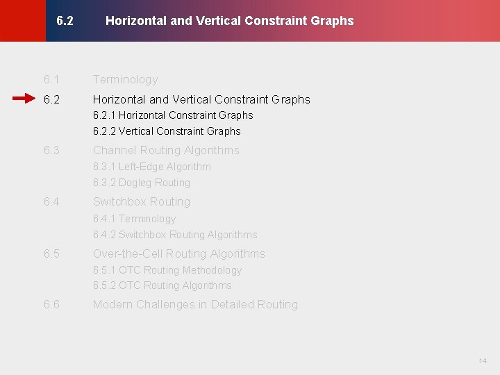
Horizontal and Vertical Constraint Graphs © KLMH 6. 2 6. 1 Terminology 6. 2 Horizontal and Vertical Constraint Graphs 6. 2. 1 Horizontal Constraint Graphs 6. 2. 2 Vertical Constraint Graphs 6. 3 Channel Routing Algorithms 6. 3. 1 Left-Edge Algorithm 6. 3. 2 Dogleg Routing 6. 4 Switchbox Routing 6. 4. 1 Terminology 6. 4. 2 Switchbox Routing Algorithms 6. 5 Over-the-Cell Routing Algorithms 6. 5. 1 OTC Routing Methodology 6. 5. 2 OTC Routing Algorithms Modern Challenges in Detailed Routing 14 Lienig 6. 6

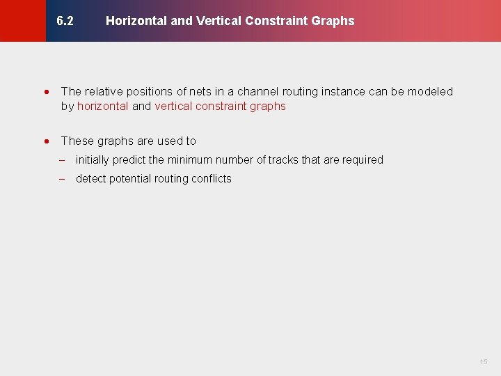
Horizontal and Vertical Constraint Graphs © KLMH 6. 2 · The relative positions of nets in a channel routing instance can be modeled by horizontal and vertical constraint graphs · These graphs are used to - initially predict the minimum number of tracks that are required 15 Lienig - detect potential routing conflicts

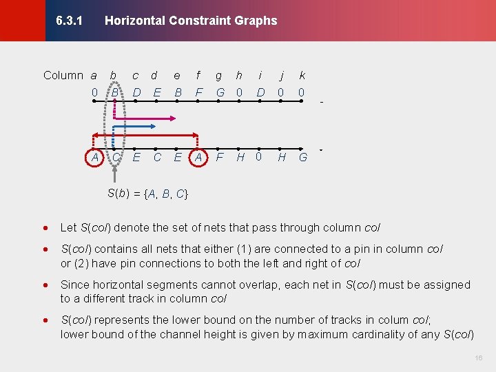
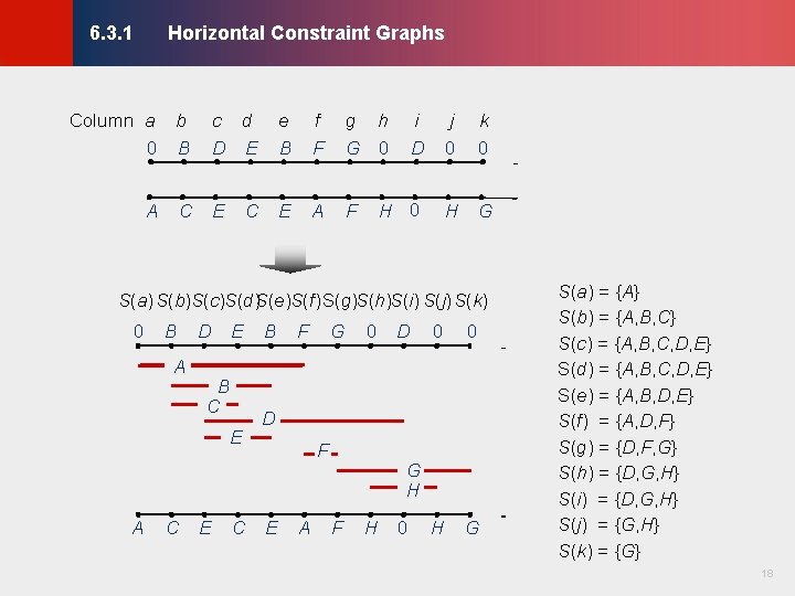
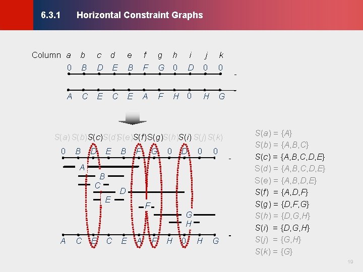
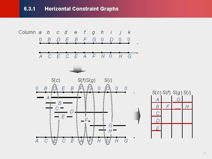
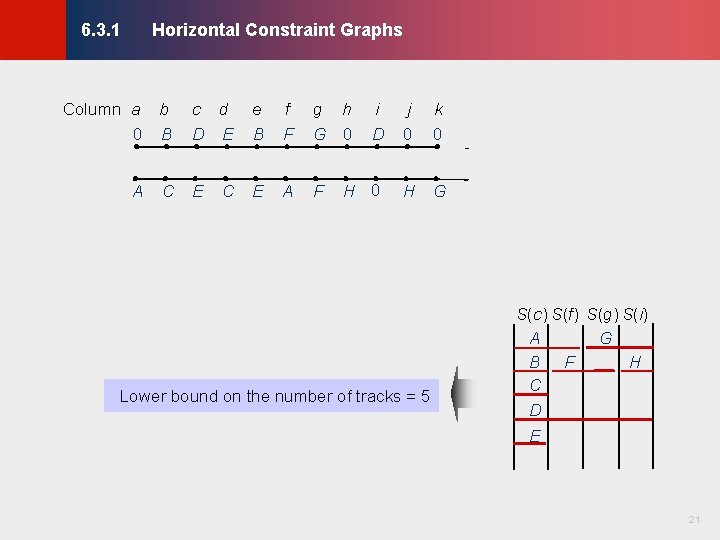
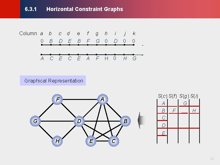
Horizontal Constraint Graphs © KLMH 6. 3. 1 Column a b 0 B A C c d D E e B f F g h G 0 E E A F C i D j 0 k 0 H G S(b) = {A, B, C} · Let S(col) denote the set of nets that pass through column col · S(col) contains all nets that either (1) are connected to a pin in column col or (2) have pin connections to both the left and right of col · Since horizontal segments cannot overlap, each net in S(col) must be assigned to a different track in column col 16 Lienig · S(col) represents the lower bound on the number of tracks in colum col; lower bound of the channel height is given by maximum cardinality of any S(col)

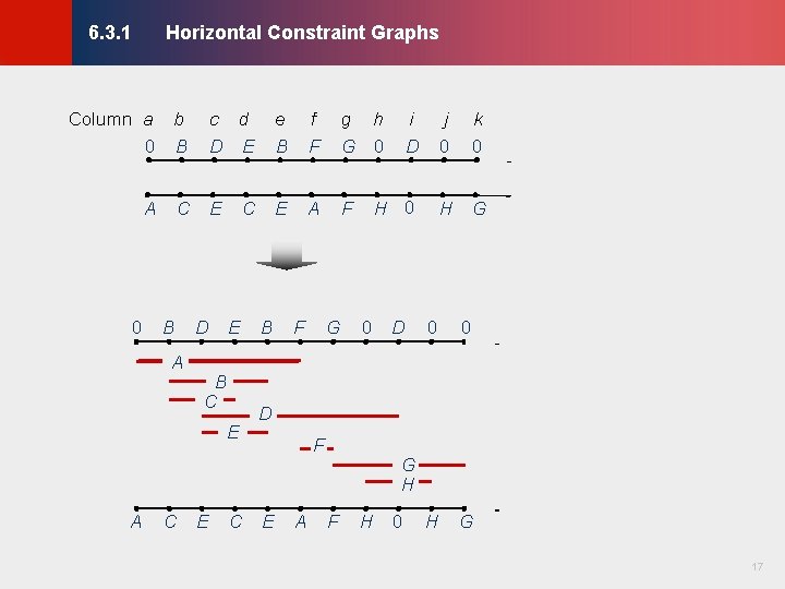
Horizontal Constraint Graphs © KLMH 6. 3. 1 A 0 C B A c d D E e B f F g h G 0 E E A F C D E B C E A C E C B F G 0 i D j 0 k 0 H G D 0 0 H G D F E A G H F H 0 17 Lienig Column a b 0 B

Horizontal Constraint Graphs © KLMH 6. 3. 1 A C c d D E e B f F g h G 0 E E A F C i D j 0 k 0 H G S(a) S(b)S(c)S(d)S(e)S(f)S(g)S(h)S(i) S(j) S(k) 0 B A D E B C E A C E C B F G 0 D 0 0 H G D F E A G H F H 0 S(a) = {A} S(b) = {A, B, C} S(c) = {A, B, C, D, E} S(d) = {A, B, C, D, E} S(e) = {A, B, D, E} S(f) = {A, D, F} S(g) = {D, F, G} S(h) = {D, G, H} S(i) = {D, G, H} S(j) = {G, H} S(k) = {G} 18 Lienig Column a b 0 B

Horizontal Constraint Graphs © KLMH 6. 3. 1 A C c d D E e B f F g h G 0 E E A F C i D j 0 k 0 H G S(a) S(b)S(c)S(d)S(e)S(f)S(g)S(h)S(i) S(j) S(k) 0 B A D E B C E A C E C B F G 0 D 0 0 H G D F E A G H F H 0 S(a) = {A} S(b) = {A, B, C} S(c) = {A, B, C, D, E} S(d) = {A, B, C, D, E} S(e) = {A, B, D, E} S(f) = {A, D, F} S(g) = {D, F, G} S(h) = {D, G, H} S(i) = {D, G, H} S(j) = {G, H} S(k) = {G} 19 Lienig Column a b 0 B

Horizontal Constraint Graphs © KLMH 6. 3. 1 A C c d D E e B f F g h G 0 E E A C S(c) 0 B A D E B C E A C E C B i D j 0 k 0 F H 0 H G S(f)S(g) S(i) F G 0 D 0 0 H G D F E A G H F H 0 S(c) S(f) S(g) S(i) A G B F H C D E 20 Lienig Column a b 0 B

Horizontal Constraint Graphs © KLMH 6. 3. 1 A C c d D E e B f F g h G 0 E E A F C i D j 0 k 0 H G Lower bound on the number of tracks = 5 S(c) S(f) S(g) S(i) A G B F H C D E 21 Lienig Column a b 0 B

Horizontal Constraint Graphs © KLMH 6. 3. 1 Column a b 0 B A C c d D E e B f F g h G 0 E E A F C i D j 0 k 0 H G Graphical Representation A G D H B E S(c) S(f) S(g) S(i) A G B F H C D E C 22 Lienig F

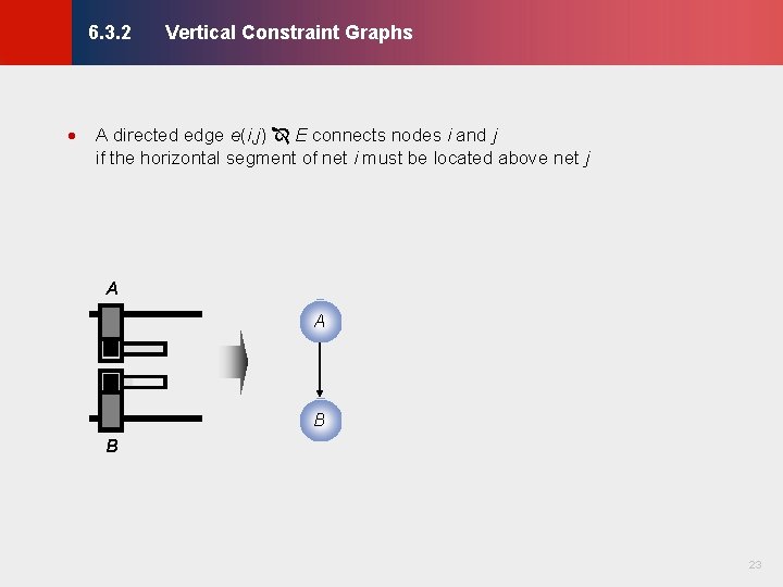
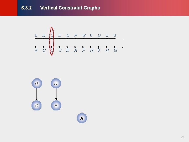
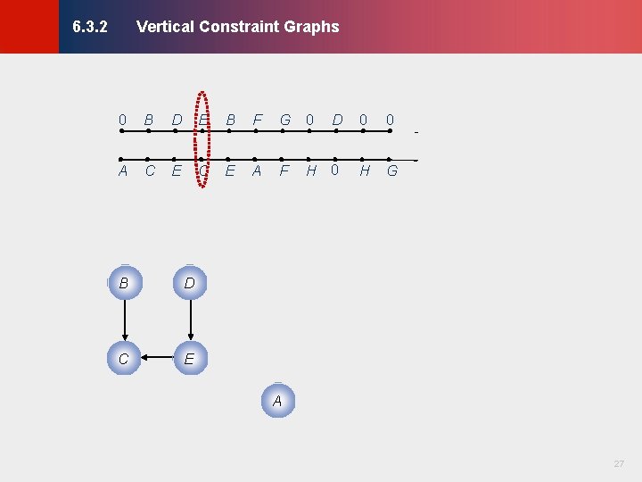
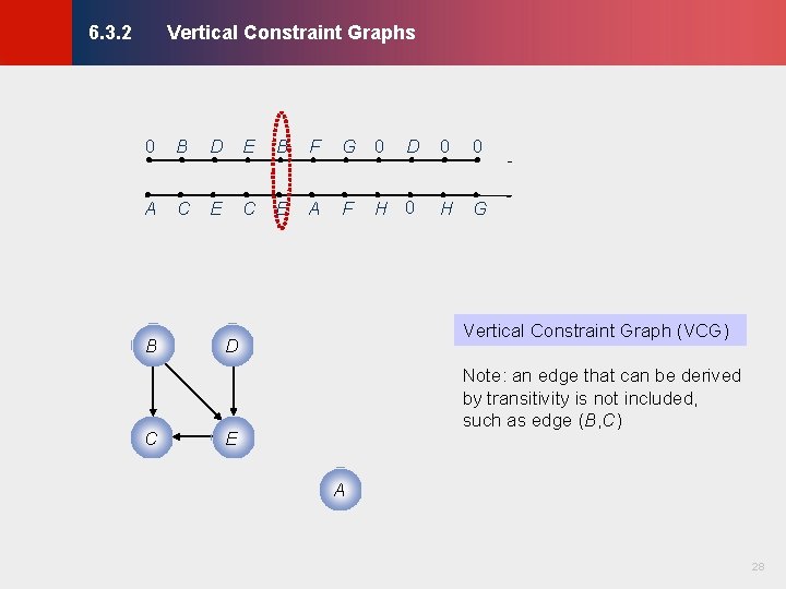
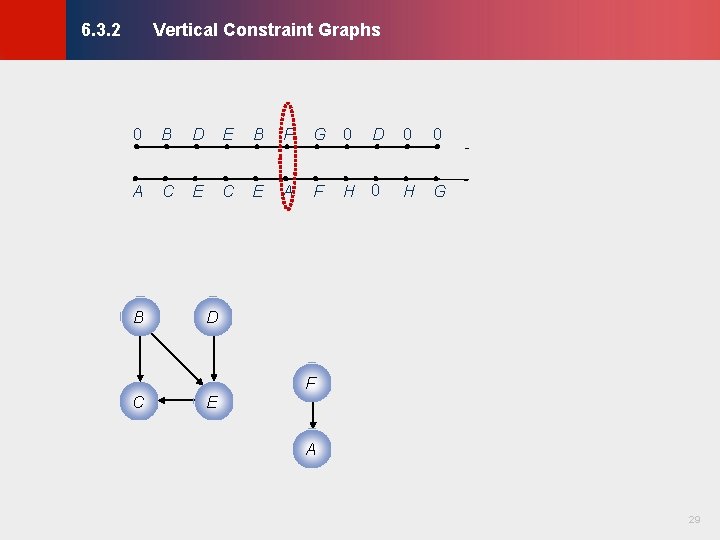
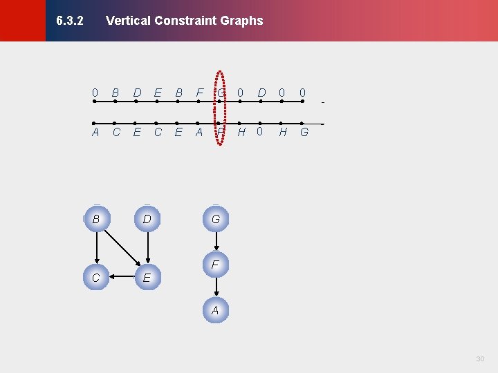
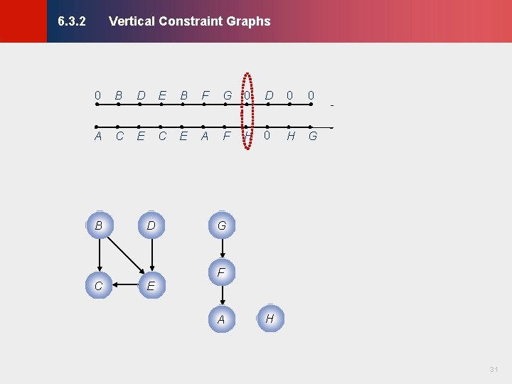
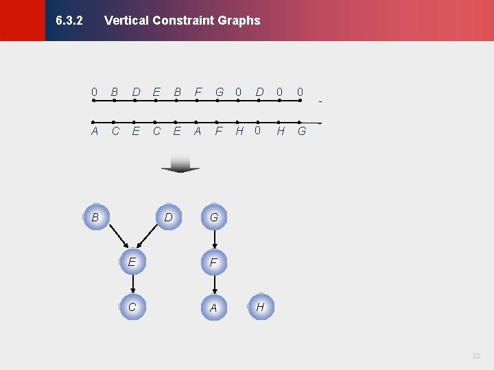
Vertical Constraint Graphs © KLMH 6. 3. 2 · A directed edge e(i, j) E connects nodes i and j if the horizontal segment of net i must be located above net j A A B 23 Lienig B

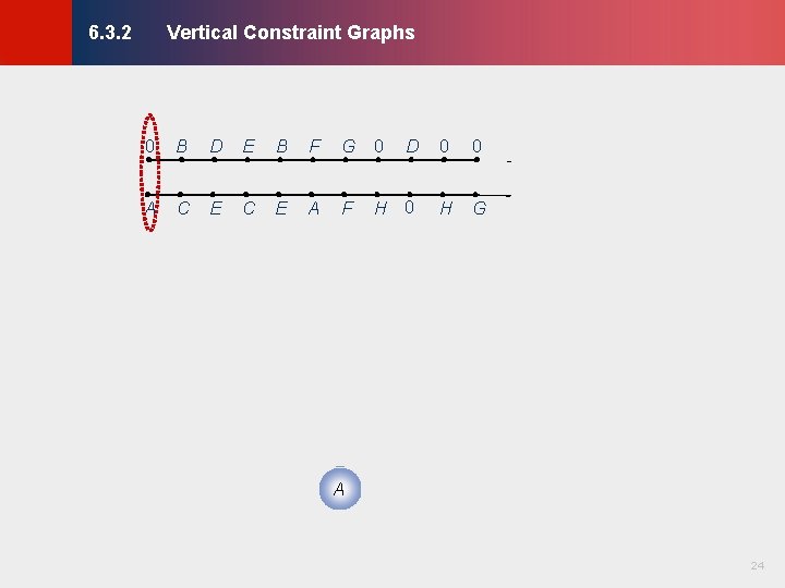
Vertical Constraint Graphs © KLMH 6. 3. 2 0 B D E B F G 0 D 0 0 A C E A F H 0 H G 24 Lienig A

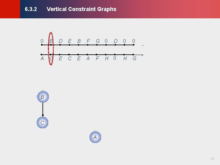
Vertical Constraint Graphs © KLMH 6. 3. 2 0 B D E B F G 0 D 0 0 A C E A F H 0 H G B C 25 Lienig A

Vertical Constraint Graphs © KLMH 6. 3. 2 0 B D E B F G 0 A C E A F D C E 0 0 H G A 26 Lienig B D

Vertical Constraint Graphs © KLMH 6. 3. 2 0 B D E B F G 0 A C E A F D C E 0 0 H G A 27 Lienig B D

Vertical Constraint Graphs © KLMH 6. 3. 2 0 B D E B F G 0 A C E A F C 0 0 H G Vertical Constraint Graph (VCG) D Note: an edge that can be derived by transitivity is not included, such as edge (B, C) E A 28 Lienig B D

Vertical Constraint Graphs © KLMH 6. 3. 2 0 B D E B F G 0 A C E A F C 0 0 H G D E F A 29 Lienig B D

Vertical Constraint Graphs © KLMH 6. 3. 2 0 B D E B F G 0 A C E A F C D E 0 0 H G G F A 30 Lienig B D

Vertical Constraint Graphs © KLMH 6. 3. 2 0 B D E B F G 0 A C E A F C D E 0 0 H G G F A H 31 Lienig B D

Vertical Constraint Graphs © KLMH 6. 3. 2 0 B D E B F G 0 A C E A F D 0 0 H G G E F C A H 32 Lienig B D

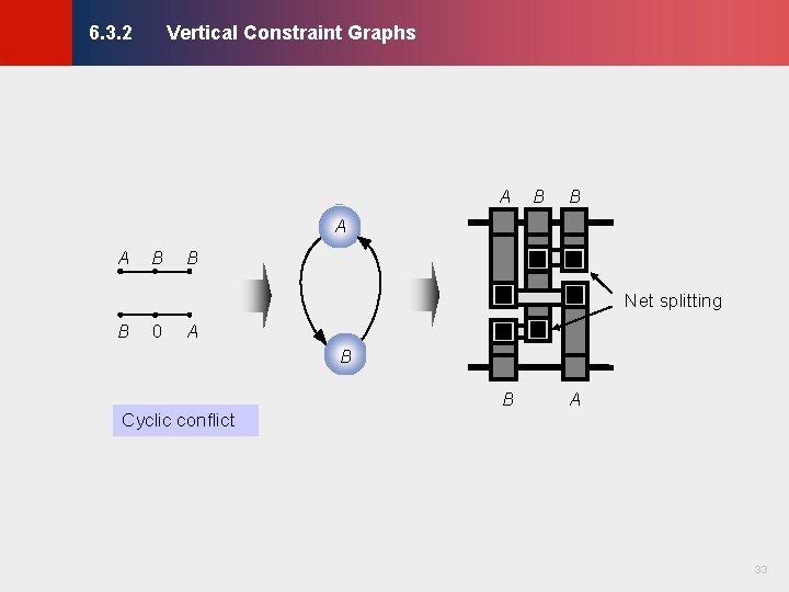
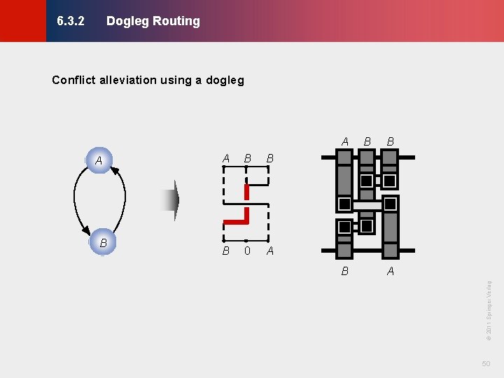
Vertical Constraint Graphs © KLMH 6. 3. 2 A B B A A B B Net splitting B 0 A B B A 33 Lienig Cyclic conflict

Channel Routing Algorithms © KLMH 6. 3 6. 1 Terminology 6. 2 Horizontal and Vertical Constraint Graphs 6. 2. 1 Horizontal Constraint Graphs 6. 2. 2 Vertical Constraint Graphs 6. 3 Channel Routing Algorithms 6. 3. 1 Left-Edge Algorithm 6. 3. 2 Dogleg Routing 6. 4 Switchbox Routing 6. 4. 1 Terminology 6. 4. 2 Switchbox Routing Algorithms 6. 5 Over-the-Cell Routing Algorithms 6. 5. 1 OTC Routing Methodology 6. 5. 2 OTC Routing Algorithms Modern Challenges in Detailed Routing 34 Lienig 6. 6

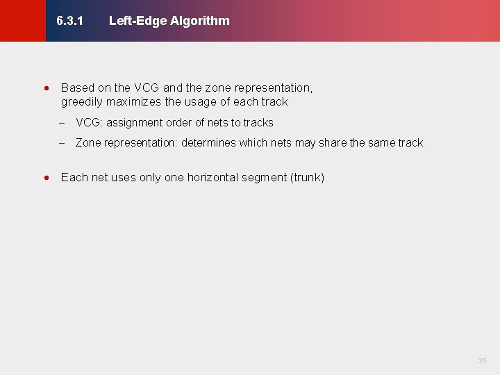
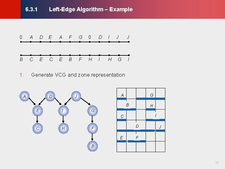
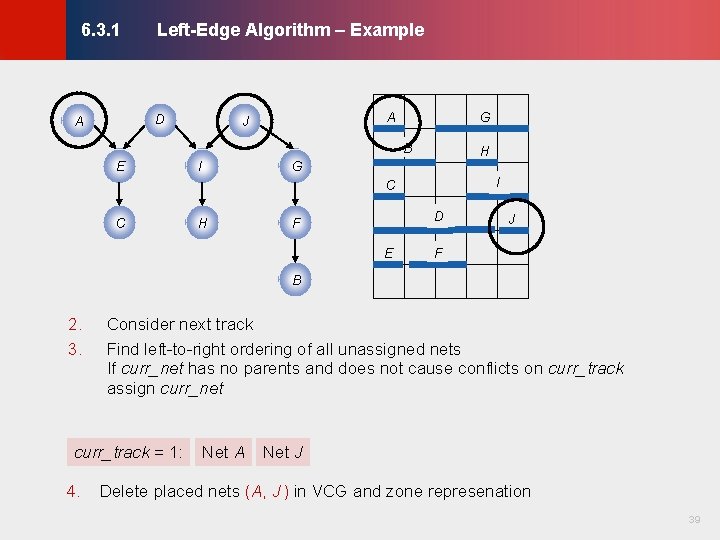
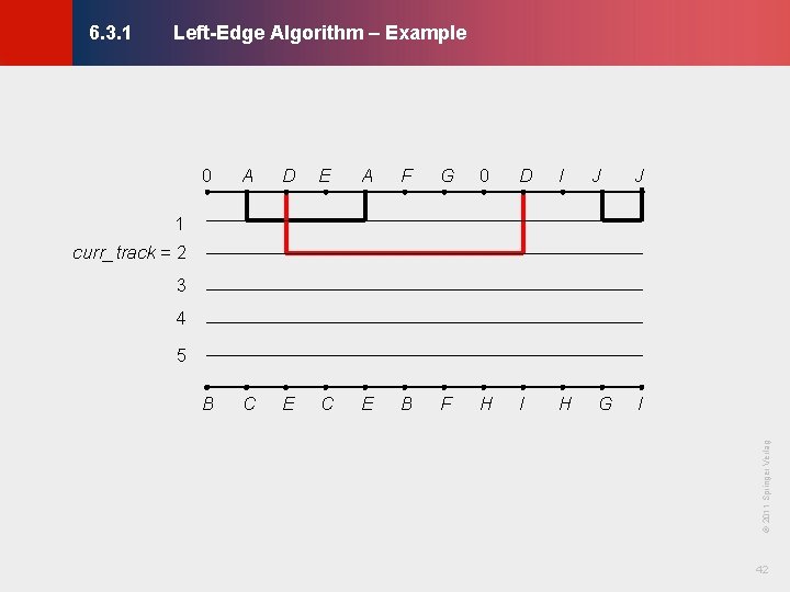
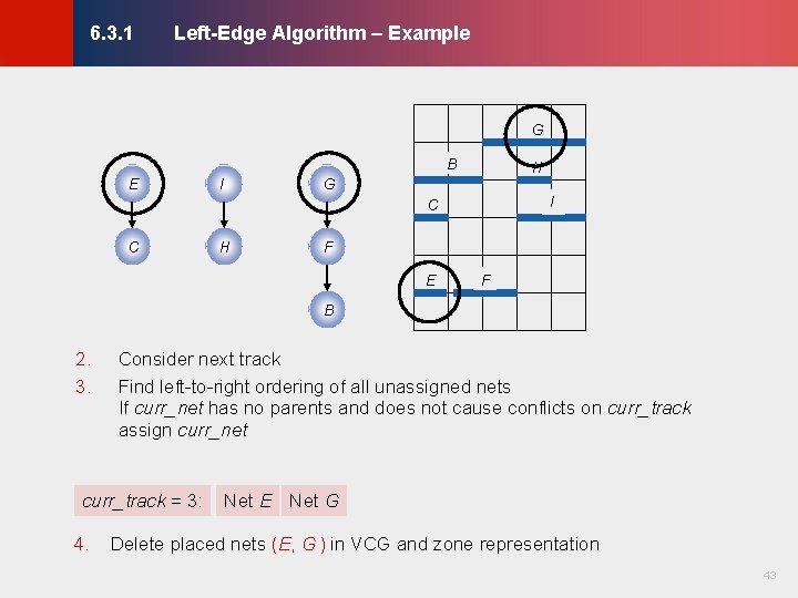
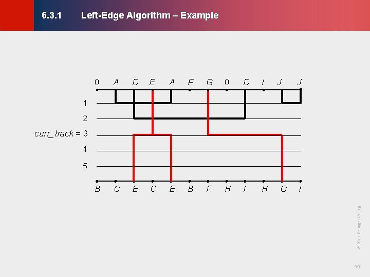
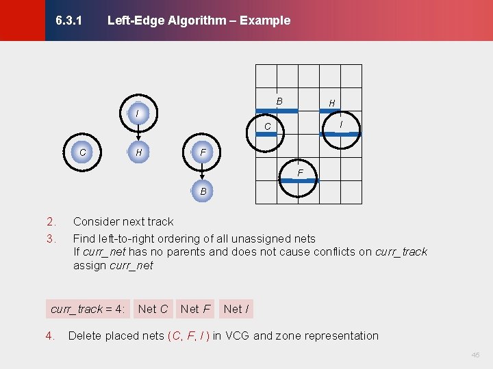
Left-Edge Algorithm © KLMH 6. 3. 1 · Based on the VCG and the zone representation, greedily maximizes the usage of each track - VCG: assignment order of nets to tracks - Zone representation: determines which nets may share the same track 35 Lienig · Each net uses only one horizontal segment (trunk)

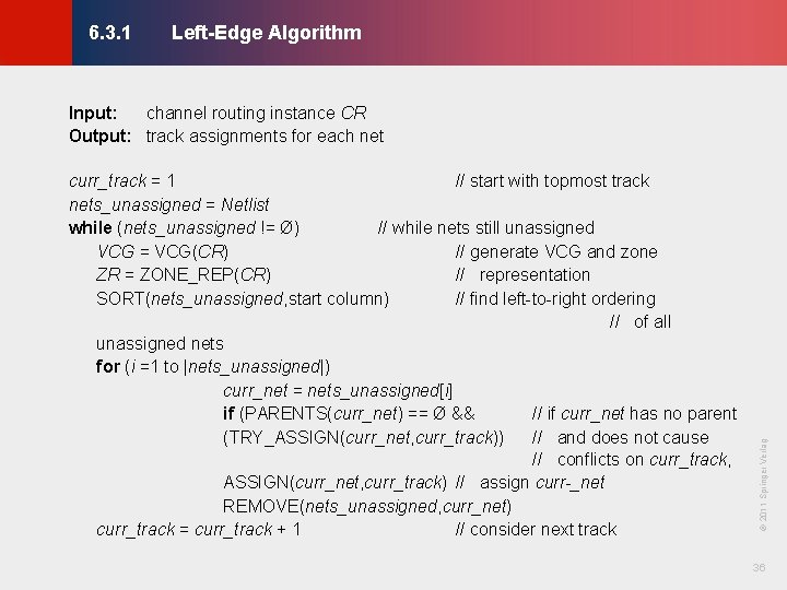
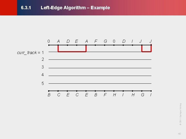
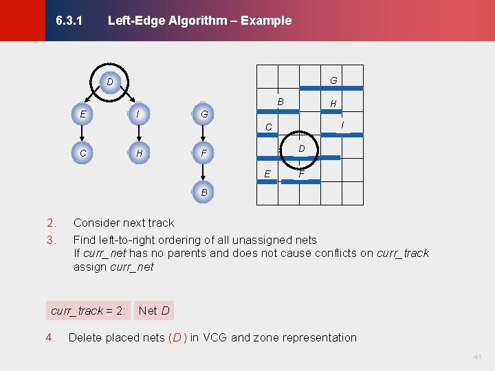
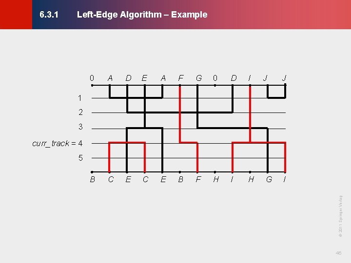
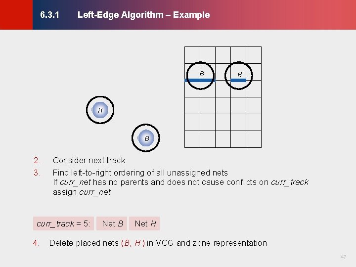
Left-Edge Algorithm © KLMH 6. 3. 1 36 Lienig curr_track = 1 // start with topmost track nets_unassigned = Netlist while (nets_unassigned != Ø) // while nets still unassigned VCG = VCG(CR) // generate VCG and zone ZR = ZONE_REP(CR) // representation SORT(nets_unassigned, start column) // find left-to-right ordering // of all unassigned nets for (i =1 to |nets_unassigned|) curr_net = nets_unassigned[i] if (PARENTS(curr_net) == Ø && // if curr_net has no parent (TRY_ASSIGN(curr_net, curr_track)) // and does not cause // conflicts on curr_track, ASSIGN(curr_net, curr_track) // assign curr _net REMOVE(nets_unassigned, curr_net) curr_track = curr_track + 1 // consider next track © 2011 Springer Verlag Input: channel routing instance CR Output: track assignments for each net

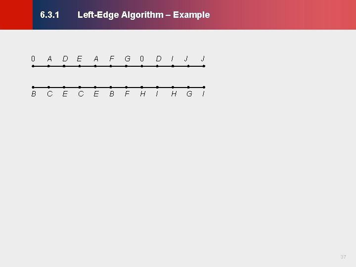
Left-Edge Algorithm – Example © KLMH 6. 3. 1 A D E A F G 0 D I B C E B F H I H J G J I 37 Lienig 0

Left-Edge Algorithm – Example © KLMH 6. 3. 1 0 A D E A F G 0 D I B C E B F H I H J G I Generate VCG and zone representation A D A J G B E I H G I C C H D F E J F B 38 Lienig 1. J

Left-Edge Algorithm – Example © KLMH 6. 3. 1 D A A J G B E I H G I C C H D F E J F B Consider next track Find left-to-right ordering of all unassigned nets If curr_net has no parents and does not cause conflicts on curr_track assign curr_net curr_track = 1: 4. Net A Net J Delete placed nets (A, J ) in VCG and zone represenation 39 Lienig 2. 3.

Left-Edge Algorithm – Example © KLMH 6. 3. 1 0 A D E A F G 0 D I B C E B F H I H J J curr_track = 1 2 3 4 5 © 2011 Springer Verlag I 40 Lienig G

Left-Edge Algorithm – Example © KLMH 6. 3. 1 G D B E I H G I C C H D F E F B Consider next track Find left-to-right ordering of all unassigned nets If curr_net has no parents and does not cause conflicts on curr_track assign curr_net curr_track = 2: 4. Net D Delete placed nets (D ) in VCG and zone representation 41 Lienig 2. 3.

Left-Edge Algorithm – Example © KLMH 6. 3. 1 0 A D E A F G 0 D I B C E B F H I H J J 1 curr_track = 2 3 4 5 © 2011 Springer Verlag I 42 Lienig G

Left-Edge Algorithm – Example © KLMH 6. 3. 1 G B E I H G I C C H F E F B Consider next track Find left-to-right ordering of all unassigned nets If curr_net has no parents and does not cause conflicts on curr_track assign curr_net curr_track = 3: 4. Net E Net G Delete placed nets (E, G ) in VCG and zone representation 43 Lienig 2. 3.

Left-Edge Algorithm – Example © KLMH 6. 3. 1 0 A D E A F G 0 D I B C E B F H I H J J 1 2 curr_track = 3 4 5 © 2011 Springer Verlag I 44 Lienig G

Left-Edge Algorithm – Example © KLMH 6. 3. 1 B H I I C C H F F B Consider next track Find left-to-right ordering of all unassigned nets If curr_net has no parents and does not cause conflicts on curr_track assign curr_net curr_track = 4: 4. Net C Net F Net I Delete placed nets (C, F, I ) in VCG and zone representation 45 Lienig 2. 3.

Left-Edge Algorithm – Example © KLMH 6. 3. 1 0 A D E A F G 0 D I B C E B F H I H J J 1 2 3 curr_track = 4 5 © 2011 Springer Verlag I 46 Lienig G

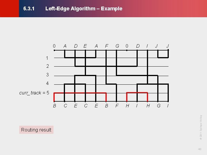
Left-Edge Algorithm – Example © KLMH 6. 3. 1 B H H B Consider next track Find left-to-right ordering of all unassigned nets If curr_net has no parents and does not cause conflicts on curr_track assign curr_net curr_track = 5: 4. Net B Net H Delete placed nets (B, H ) in VCG and zone representation 47 Lienig 2. 3.

Left-Edge Algorithm – Example © KLMH 6. 3. 1 0 A D E A F G 0 D I B C E B F H I H J J 1 2 3 4 curr_track = 5 © 2011 Springer Verlag I 48 Lienig Routing result G

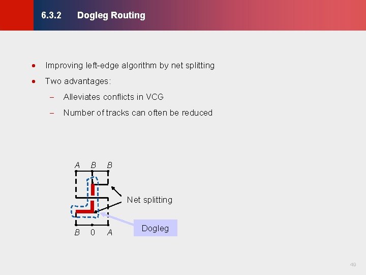
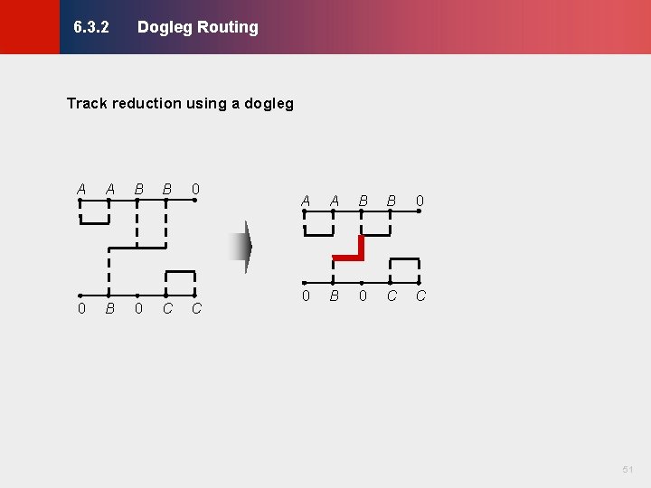
Dogleg Routing © KLMH 6. 3. 2 · Improving left-edge algorithm by net splitting · Two advantages: - Alleviates conflicts in VCG - Number of tracks can often be reduced A B B Net splitting 0 A Dogleg 49 Lienig B

Dogleg Routing © KLMH 6. 3. 2 Conflict alleviation using a dogleg B A B B B 0 A B B A © 2011 Springer Verlag A B 50 Lienig A

Dogleg Routing © KLMH 6. 3. 2 A A B B 0 0 B 0 C C 51 Lienig Track reduction using a dogleg

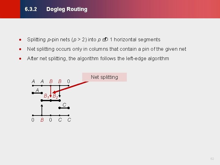
Dogleg Routing © KLMH 6. 3. 2 · Splitting p-pin nets (p > 2) into p 1 horizontal segments · Net splitting occurs only in columns that contain a pin of the given net · After net splitting, the algorithm follows the left-edge algorithm A A A B 0 B Net splitting B 1 B 2 C B 0 C C 52 Lienig 0

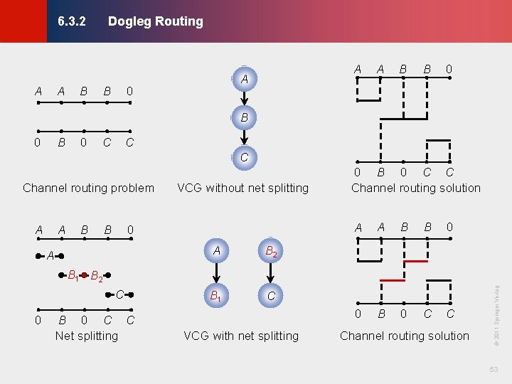
Dogleg Routing © KLMH 6. 3. 2 A A B B A A 0 A B B 0 B 0 C Channel routing problem A A B B VCG without net splitting 0 A A B 2 B 1 C 0 B 0 C C Channel routing solution A A B B 0 0 B 0 C C Net splitting VCG with net splitting Channel routing solution 53 Lienig C © 2011 Springer Verlag B 1 B 2

Switchbox Routing © KLMH 6. 4 6. 1 Terminology 6. 2 Horizontal and Vertical Constraint Graphs 6. 2. 1 Horizontal Constraint Graphs 6. 2. 2 Vertical Constraint Graphs 6. 3 Channel Routing Algorithms 6. 3. 1 Left-Edge Algorithm 6. 3. 2 Dogleg Routing 6. 4 Switchbox Routing 6. 4. 1 Terminology 6. 4. 2 Switchbox Routing Algorithms 6. 5 Over-the-Cell Routing Algorithms 6. 5. 1 OTC Routing Methodology 6. 5. 2 OTC Routing Algorithms Modern Challenges in Detailed Routing 54 Lienig 6. 6

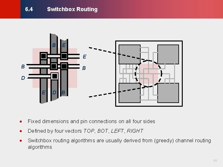
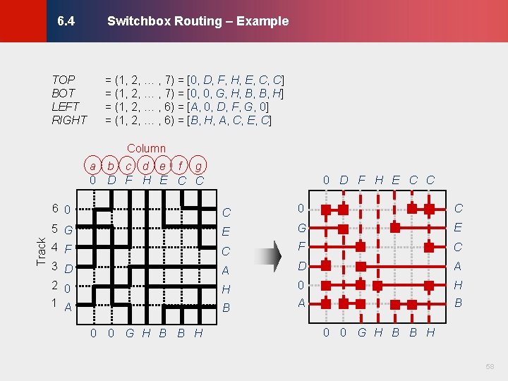
Switchbox Routing © KLMH 6. 4 B E E B B D D B · Fixed dimensions and pin connections on all four sides · Defined by four vectors TOP, BOT, LEFT, RIGHT · Switchbox routing algorithms are usually derived from (greedy) channel routing algorithms 55 Lienig E

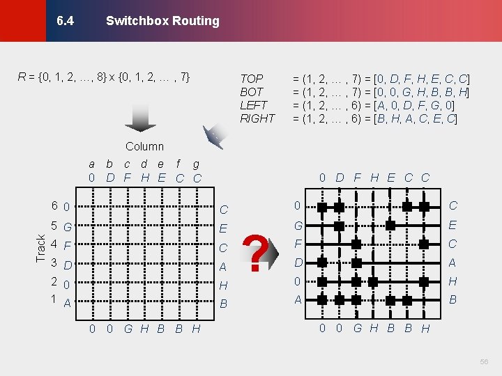
Switchbox Routing © KLMH 6. 4 R = {0, 1, 2, …, 8} x {0, 1, 2, … , 7} TOP BOT LEFT RIGHT = (1, 2, … , 7) = [0, D, F, H, E, C, C] = (1, 2, … , 7) = [0, 0, G, H, B, B, H] = (1, 2, … , 6) = [A, 0, D, F, G, 0] = (1, 2, … , 6) = [B, H, A, C, E, C] Column 0 D F H E C C 6 0 C 5 G 4 F E G E F C 3 D 2 0 A D A 0 H 1 A B C H 0 0 G H B B H ? 0 0 G H B B H 56 Lienig Track a b c d e f g 0 D F H E C C

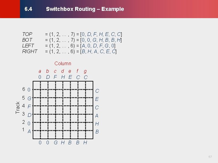
Switchbox Routing – Example TOP BOT LEFT RIGHT = (1, 2, … , 7) = [0, D, F, H, E, C, C] = (1, 2, … , 7) = [0, 0, G, H, B, B, H] = (1, 2, … , 6) = [A, 0, D, F, G, 0] = (1, 2, … , 6) = [B, H, A, C, E, C] © KLMH 6. 4 Column 6 0 C 5 G 4 F E 3 D 2 0 A 1 A B C H 0 0 G H B B H 57 Lienig Track a b c d e f g 0 D F H E C C

Switchbox Routing – Example TOP BOT LEFT RIGHT = (1, 2, … , 7) = [0, D, F, H, E, C, C] = (1, 2, … , 7) = [0, 0, G, H, B, B, H] = (1, 2, … , 6) = [A, 0, D, F, G, 0] = (1, 2, … , 6) = [B, H, A, C, E, C] © KLMH 6. 4 Column 0 D F H E C C 6 0 C 5 G 4 F E G E C F C 3 D 2 0 A D A H 0 H 1 A B 0 0 G H B B H 58 Lienig Track a b c d e f g 0 D F H E C C

Over-the-Cell Routing Algorithms © KLMH 6. 5 6. 1 Terminology 6. 2 Horizontal and Vertical Constraint Graphs 6. 2. 1 Horizontal Constraint Graphs 6. 2. 2 Vertical Constraint Graphs 6. 3 Channel Routing Algorithms 6. 3. 1 Left-Edge Algorithm 6. 3. 2 Dogleg Routing 6. 4 Switchbox Routing 6. 4. 1 Terminology 6. 4. 2 Switchbox Routing Algorithms 6. 5 Over-the-Cell Routing Algorithms 6. 5. 1 OTC Routing Methodology 6. 5. 2 OTC Routing Algorithms Modern Challenges in Detailed Routing 59 Lienig 6. 6

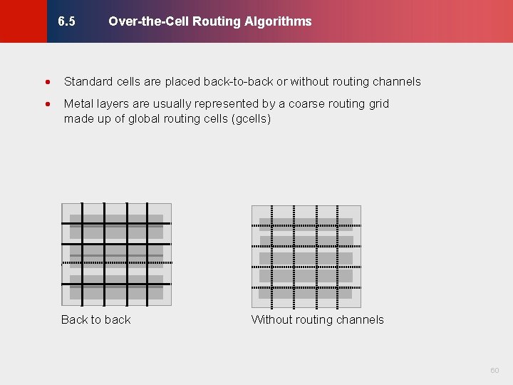
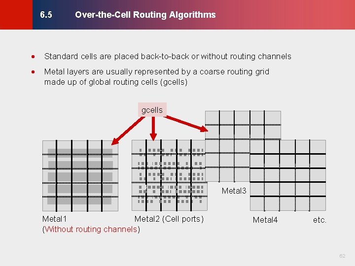
Over-the-Cell Routing Algorithms © KLMH 6. 5 · Standard cells are placed back-to-back or without routing channels · Metal layers are usually represented by a coarse routing grid made up of global routing cells (gcells) Without routing channels 60 Lienig Back to back

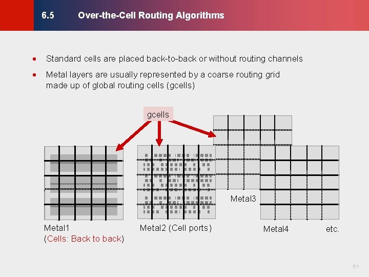
Over-the-Cell Routing Algorithms © KLMH 6. 5 · Standard cells are placed back-to-back or without routing channels · Metal layers are usually represented by a coarse routing grid made up of global routing cells (gcells) gcells Metal 3 Metal 2 (Cell ports) Metal 4 etc. 61 Lienig Metal 1 (Cells: Back to back)

Over-the-Cell Routing Algorithms © KLMH 6. 5 · Standard cells are placed back-to-back or without routing channels · Metal layers are usually represented by a coarse routing grid made up of global routing cells (gcells) gcells Metal 3 Metal 4 etc. 62 Lienig Metal 1 Metal 2 (Cell ports) (Without routing channels)

Over-the-Cell Routing Algorithms · Standard cells are placed back-to-back or without routing channels · Metal layers are usually represented by a coarse routing grid made up of global routing cells (gcells) · Layers that are not obstructed by standard cells are typically used for over-the-cell (OTC) routing · Nets are globally routed using gcells and then detail-routed 63 Lienig © KLMH 6. 5

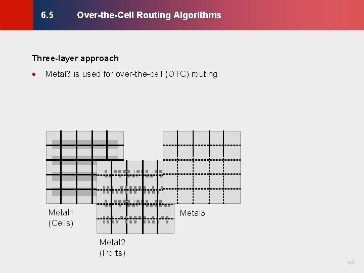
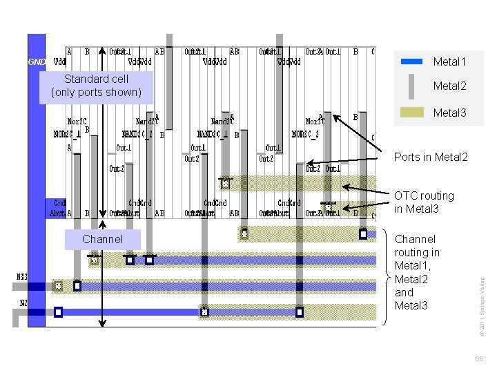
Over-the-Cell Routing Algorithms © KLMH 6. 5 Three-layer approach Metal 3 is used for over-the-cell (OTC) routing Metal 1 (Cells) Metal 3 Metal 2 (Ports) 64 Lienig ·

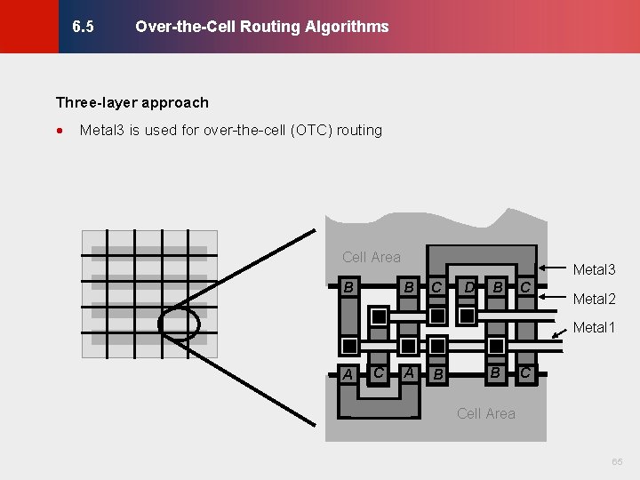
Over-the-Cell Routing Algorithms © KLMH 6. 5 Three-layer approach Metal 3 is used for over-the-cell (OTC) routing Cell Area B Metal 3 B C D B C Metal 2 Metal 1 A C A B B C Cell Area 65 Lienig ·

Standard cell (only ports shown) © KLMH Metal 1 GND Metal 2 Metal 3 Ports in Metal 2 Channel routing in Metal 1, Metal 2 and Metal 3 66 Lienig Channel © 2011 Springer Verlag OTC routing in Metal 3

Modern Challenges in Detailed Routing © KLMH 6. 6 6. 1 Terminology 6. 2 Horizontal and Vertical Constraint Graphs 6. 2. 1 Horizontal Constraint Graphs 6. 2. 2 Vertical Constraint Graphs 6. 3 Channel Routing Algorithms 6. 3. 1 Left-Edge Algorithm 6. 3. 2 Dogleg Routing 6. 4 Switchbox Routing 6. 4. 1 Terminology 6. 4. 2 Switchbox Routing Algorithms 6. 5 Over-the-Cell Routing Algorithms 6. 5. 1 OTC Routing Methodology 6. 5. 2 OTC Routing Algorithms Modern Challenges in Detailed Routing 67 Lienig 6. 6

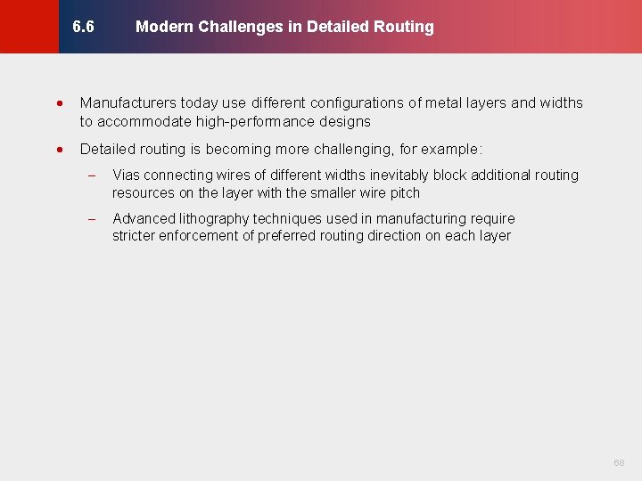
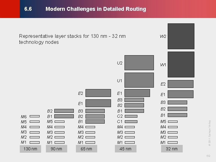
Modern Challenges in Detailed Routing · Manufacturers today use different configurations of metal layers and widths to accommodate high-performance designs · Detailed routing is becoming more challenging, for example: - Vias connecting wires of different widths inevitably block additional routing resources on the layer with the smaller wire pitch - Advanced lithography techniques used in manufacturing require stricter enforcement of preferred routing direction on each layer 68 Lienig © KLMH 6. 6

Modern Challenges in Detailed Routing © KLMH 6. 6 U 1 E 2 E 1 M 6 M 5 M 4 M 3 M 2 M 1 130 nm B 2 B 1 M 5 M 4 M 3 M 2 M 1 90 nm B 3 B 2 B 1 M 4 M 3 M 2 M 1 65 nm E 1 B 3 B 2 B 1 C 2 C 1 M 4 M 3 M 2 M 1 45 nm W 1 E 2 E 1 B 3 B 2 B 1 M 5 M 4 M 3 M 2 M 1 © 2011 Springer Verlag U 2 W 2 32 nm 69 Lienig Representative layer stacks for 130 nm - 32 nm technology nodes

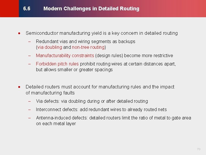
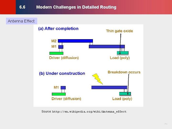
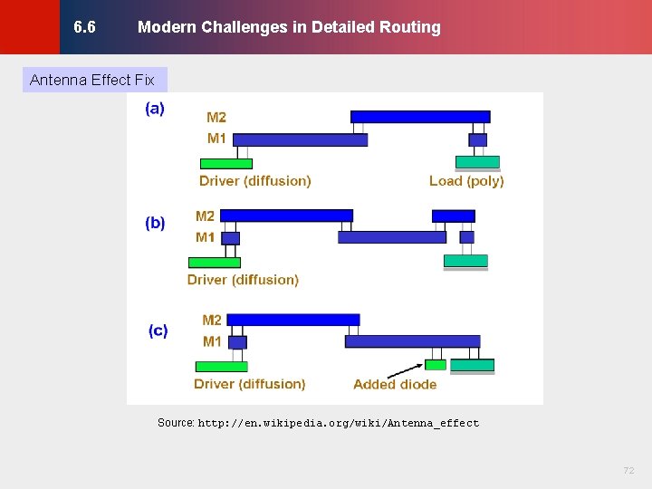
Modern Challenges in Detailed Routing © KLMH 6. 6 · Semiconductor manufacturing yield is a key concern in detailed routing - Redundant vias and wiring segments as backups (via doubling and non-tree routing) - Manufacturability constraints (design rules) become more restrictive - Forbidden pitch rules prohibit routing wires at certain distances apart, but allows smaller or greater spacings Detailed routers must account for manufacturing rules and the impact of manufacturing faults - Via defects: via doubling during or after detailed routing - Interconnect defects: add redundant wires to already routed nets - Antenna-induced defects: detailed routers limit the ratio of metal to gate area on each metal layer 70 Lienig ·

© KLMH Modern Challenges in Detailed Routing Antenna Effect Source: http: //en. wikipedia. org/wiki/Antenna_effect 71 Lienig 6. 6

© KLMH Modern Challenges in Detailed Routing Antenna Effect Fix Source: http: //en. wikipedia. org/wiki/Antenna_effect 72 Lienig 6. 6

© KLMH Summary of Chapter 6 – Context · Detailed routing is invoked after global routing · Usually takes about as much time as global routing - · Generates specific track assignments for each connection - Tries to follow "suggestions" made by global routing, but may alter them if necessary - A small number of failed global routed (disconnected, overcapacity) can be tolerated More affected by technology & manufacturing constraints than global routing - Must satisfy design rules 73 Lienig · For heavily congested designs can take much longer

© KLMH Summary of Chapter 6 – Routing Regions · · Breaks down the layout area into regions - Channels have net terminals (pins) on two sides - Switch-boxes have terminals on four sides - Channels are joined at switchboxes When the number of metal layers is >3, use over-the-cell (OTC) routing - Divide the layout region into a grid of global routing cells (gcells) - OTC routing makes the locations of cells, obstacles and pins less important - Channel and switchbox routing can be used during OTC routing when upper metal layers are blocked (by wide buses, other wires, etc. ) The capacity of a region is limited by the number of tracks it contains - Channels, switchboxes, gcells 74 Lienig ·

· Horizontal and vertical constraint graphs capture constraints that must be satisfied by valid routes · Simplest algorithms for detailed routing are greedy - Every step satisfies immediate constraints with minimal routing cost - Use as few bends as possible (doglegs are used when additional bends are needed) - Very fast, do a surprisingly good job in many cases - Insufficient for congested designs · Switchbox routing algorithms are usually derived from channel routing algorithms · Strategy 1: Do not create congested designs and rely on greedy algorithms · Strategy 2: Accommodate congested designs and develop stronger algorithms 75 Lienig © KLMH Summary of Chapter 6 – Algorithms and Data Structures

© KLMH Summary of Chapter 6 – Modern Challenges Variable-pitch wire stacks - · · · Satisfying more complex design rules - Min spacing between wires and devices - Forbidden pitch rules - Antenna rules Soft rules - Do not need to be satisfied - Can improve yield by decreasing the probability of defects Redundant vias - · Not addressed in the literature until 2008 In case some vias are poorly manufactured Redundant wires - In case some wires get disconnected 76 Lienig ·