Introduction to Survival Analysis Kristin Sainani Ph D

Introduction to Survival Analysis Kristin Sainani Ph. D. http: //www. stanford. edu/~kcobb Stanford University Department of Health Research and Policy 1

Overview n n n What is survival analysis? Terminology and data structure. Survival/hazard functions. Parametric versus semi-parametric regression techniques. Introduction to Kaplan-Meier methods (non-parametric). Relevant SAS Procedures (PROCS). 2

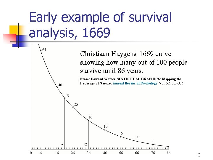
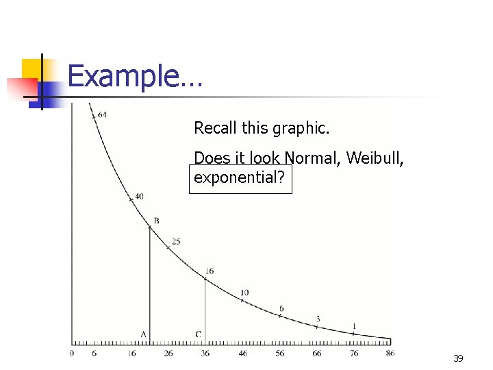
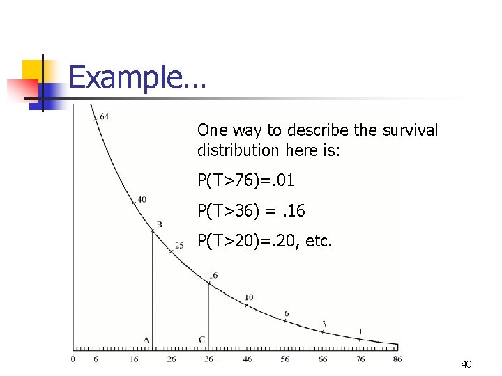
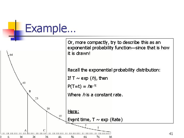
Early example of survival analysis, 1669 Christiaan Huygens' 1669 curve showing how many out of 100 people survive until 86 years. From: Howard Wainer STATISTICAL GRAPHICS: Mapping the Pathways of Science. Annual Review of Psychology. Vol. 52: 305 -335. 3

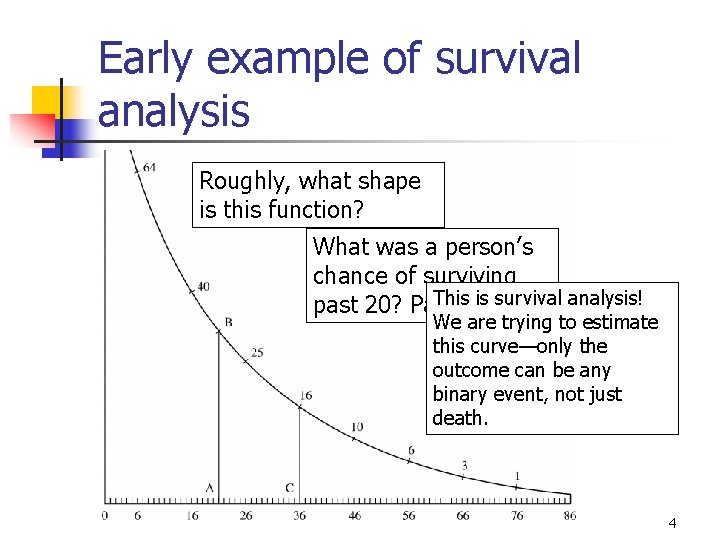
Early example of survival analysis Roughly, what shape is this function? What was a person’s chance of surviving This 36? is survival analysis! past 20? Past We are trying to estimate this curve—only the outcome can be any binary event, not just death. 4

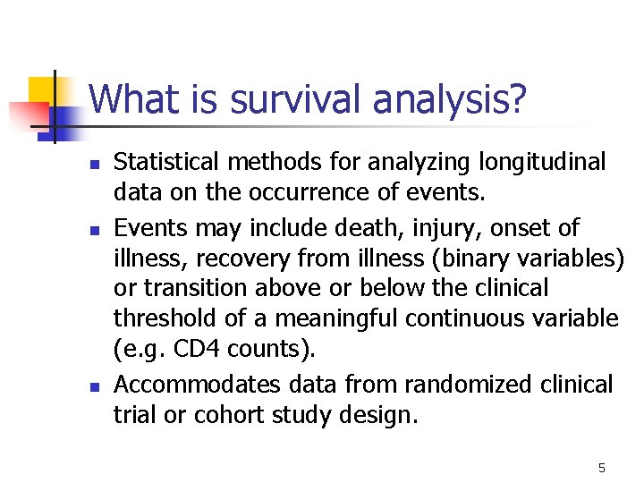
What is survival analysis? n n n Statistical methods for analyzing longitudinal data on the occurrence of events. Events may include death, injury, onset of illness, recovery from illness (binary variables) or transition above or below the clinical threshold of a meaningful continuous variable (e. g. CD 4 counts). Accommodates data from randomized clinical trial or cohort study design. 5

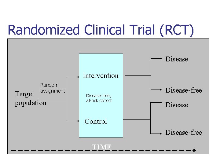
Randomized Clinical Trial (RCT) Disease Intervention Random assignment Target population Disease-free, at-risk cohort Disease-free Disease Control Disease-free TIME

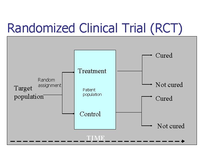
Randomized Clinical Trial (RCT) Cured Treatment Random assignment Target population Patient population Not cured Control Not cured TIME

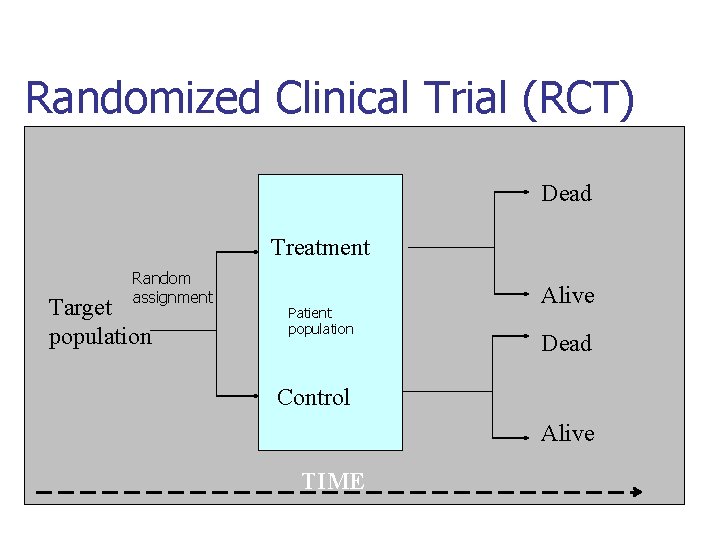
Randomized Clinical Trial (RCT) Dead Treatment Random assignment Target population Patient population Alive Dead Control Alive TIME

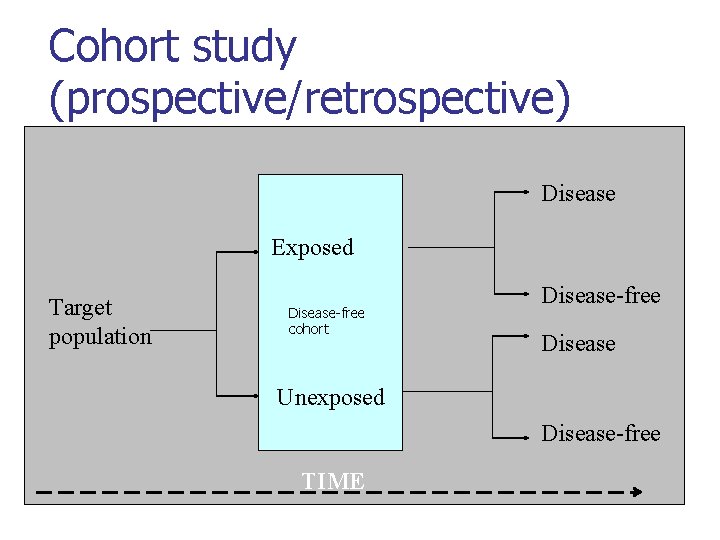
Cohort study (prospective/retrospective) Disease Exposed Target population Disease-free cohort Disease-free Disease Unexposed Disease-free TIME

Examples of survival analysis in medicine 10

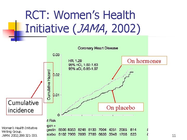
RCT: Women’s Health Initiative (JAMA, 2002) On hormones Cumulative incidence Women’s Health Initiative Writing Group. JAMA. 2002; 288: 321 -333. On placebo 11

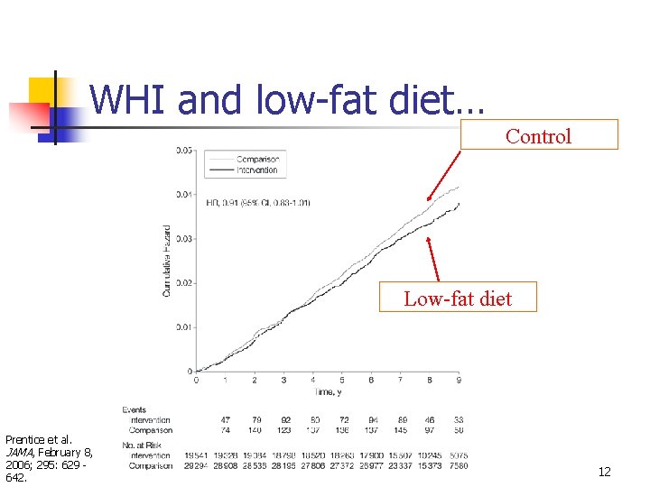
WHI and low-fat diet… Control Low-fat diet Prentice et al. JAMA, February 8, 2006; 295: 629 642. 12

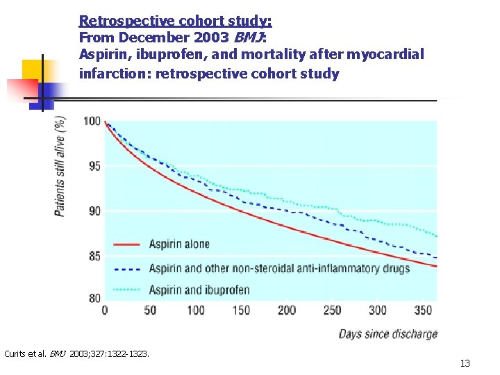
Retrospective cohort study: From December 2003 BMJ: Aspirin, ibuprofen, and mortality after myocardial infarction: retrospective cohort study Curits et al. BMJ 2003; 327: 1322 -1323. 13

Objectives of survival analysis Estimate time-to-event for a group of individuals, such as time until second heartattack for a group of MI patients. n To compare time-to-event between two or more groups, such as treated vs. placebo MI patients in a randomized controlled trial. n To assess the relationship of co-variables to time-to-event, such as: does weight, insulin resistance, or cholesterol influence survival time of MI patients? Note: expected time-to-event = 1/incidence rate n 14

Why use survival analysis? 1. Why not compare mean time-to-event between your groups using a t-test or linear regression? -- ignores censoring 2. Why not compare proportion of events in your groups using risk/odds ratios or logistic regression? --ignores time 15

Survival Analysis: Terms n n Time-to-event: The time from entry into a study until a subject has a particular outcome Censoring: Subjects are said to be censored if they are lost to follow up or drop out of the study, or if the study ends before they die or have an outcome of interest. They are counted as alive or disease-free for the time they were enrolled in the study. n If dropout is related to both outcome and treatment, dropouts may bias the results 16

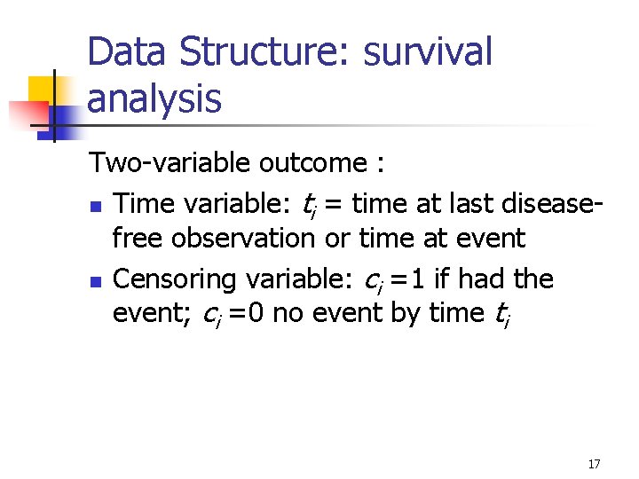
Data Structure: survival analysis Two-variable outcome : n Time variable: ti = time at last diseasefree observation or time at event n Censoring variable: ci =1 if had the event; ci =0 no event by time ti 17

Right Censoring (T>t) Common examples n Termination of the study n Death due to a cause that is not the event of interest n Loss to follow-up We know that subject survived at least to time t. 18

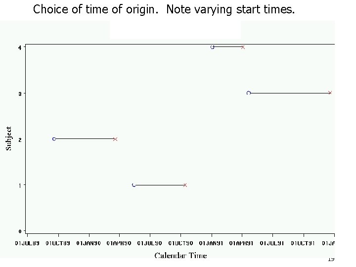
Choice of time of origin. Note varying start times. 19

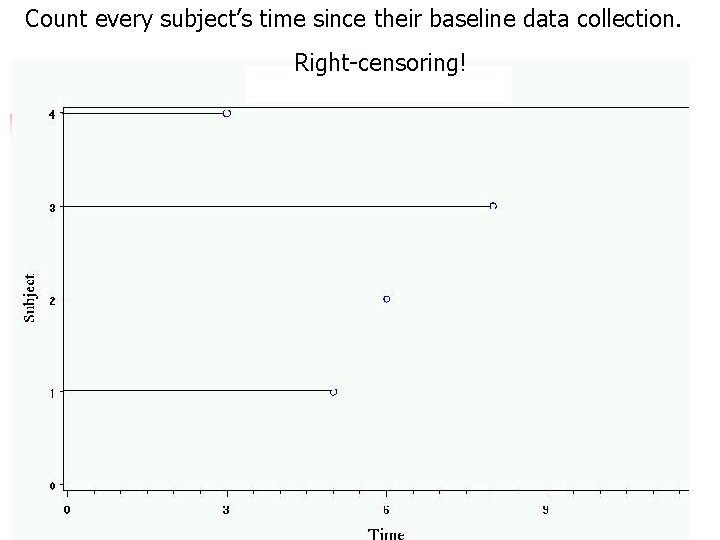
Count every subject’s time since their baseline data collection. Right-censoring! 20

Introduction to survival distributions n n Ti the event time for an individual, is a random variable having a probability distribution. Different models for survival data are distinguished by different choice of distribution for Ti. 21

Describing Survival Distributions Parametric survival analysis is based on so-called “Waiting Time” distributions (ex: exponential probability distribution). The idea is this: Assume that times-to-event for individuals in your dataset follow a continuous probability distribution (which we may or may not be able to pin down mathematically). For all possible times Ti after baseline, there is a certain probability that an individual will have an event at exactly time Ti. For example, human beings have a certain probability of dying at ages 3, 25, 80, and 140: P(T=3), P(T=25), P(T=80), P(T=140). These probabilities are obviously vastly different. 22

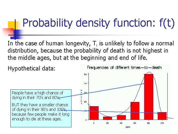
Probability density function: f(t) In the case of human longevity, Ti is unlikely to follow a normal distribution, because the probability of death is not highest in the middle ages, but at the beginning and end of life. Hypothetical data: People have a high chance of dying in their 70’s and 80’s; BUT they have a smaller chance of dying in their 90’s and 100’s, because few people make it long enough to die at these ages. 23

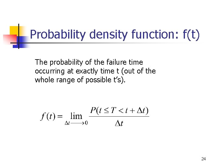
Probability density function: f(t) The probability of the failure time occurring at exactly time t (out of the whole range of possible t’s). 24

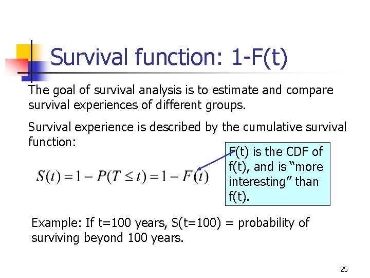
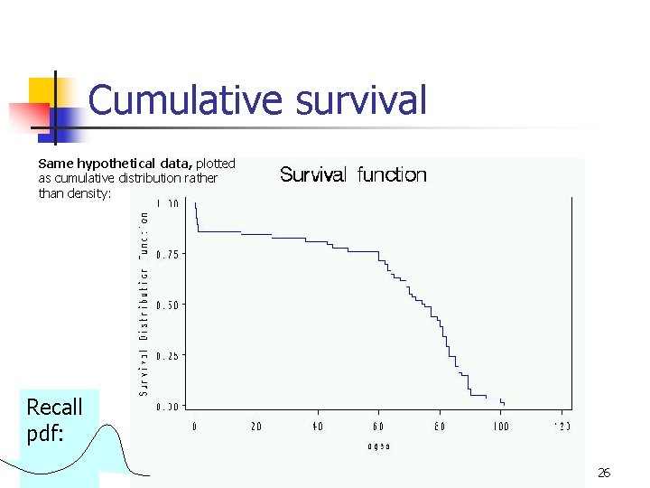
Survival function: 1 -F(t) The goal of survival analysis is to estimate and compare survival experiences of different groups. Survival experience is described by the cumulative survival function: F(t) is the CDF of f(t), and is “more interesting” than f(t). Example: If t=100 years, S(t=100) = probability of surviving beyond 100 years. 25

Cumulative survival Same hypothetical data, plotted as cumulative distribution rather than density: Recall pdf: 26

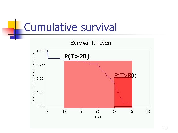
Cumulative survival P(T>20) P(T>80) 27

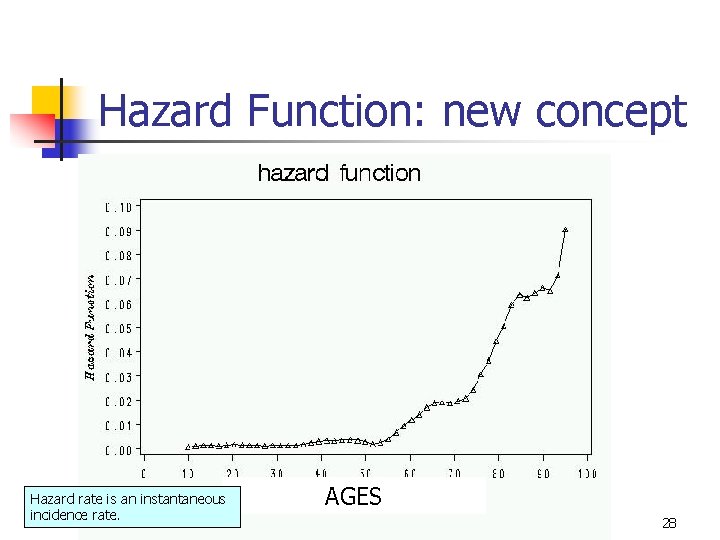
Hazard Function: new concept Hazard rate is an instantaneous incidence rate. AGES 28

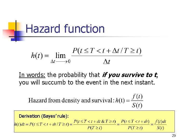
Hazard function In words: the probability that if you survive to t, you will succumb to the event in the next instant. Derivation (Bayes’ rule): 29

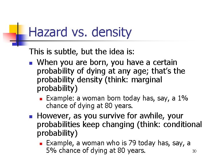
Hazard vs. density This is subtle, but the idea is: n When you are born, you have a certain probability of dying at any age; that’s the probability density (think: marginal probability) n n Example: a woman born today has, say, a 1% chance of dying at 80 years. However, as you survive for awhile, your probabilities keep changing (think: conditional probability) n Example, a woman who is 79 today has, say, a 30 5% chance of dying at 80 years.

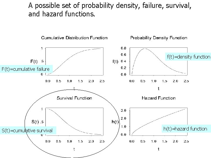
A possible set of probability density, failure, survival, and hazard functions. f(t)=density function F(t)=cumulative failure S(t)=cumulative survival h(t)=hazard function 31

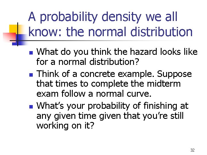
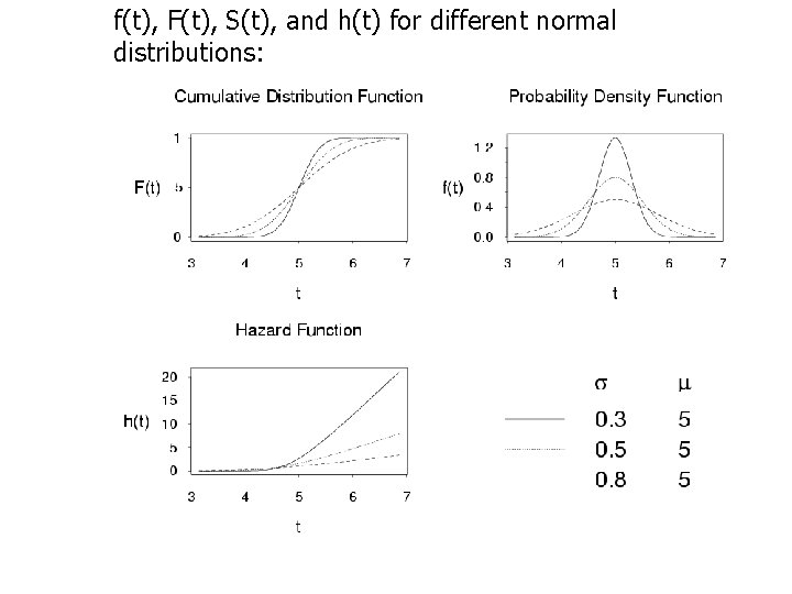
A probability density we all know: the normal distribution n What do you think the hazard looks like for a normal distribution? Think of a concrete example. Suppose that times to complete the midterm exam follow a normal curve. What’s your probability of finishing at any given time given that you’re still working on it? 32

f(t), F(t), S(t), and h(t) for different normal distributions: 33

Examples: common functions to describe survival n n Exponential (hazard is constant over time, simplest!) Weibull (hazard function is increasing or decreasing over time) 34

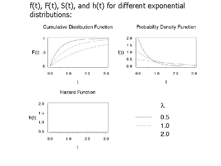
f(t), F(t), S(t), and h(t) for different exponential distributions: 35

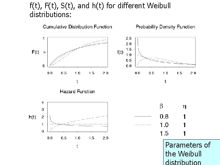
f(t), F(t), S(t), and h(t) for different Weibull distributions: Parameters of the Weibull 36

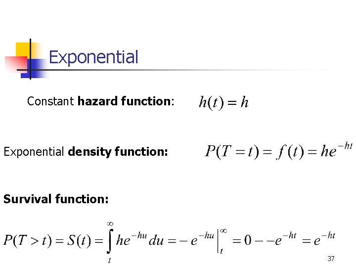
Exponential Constant hazard function: Exponential density function: Survival function: 37

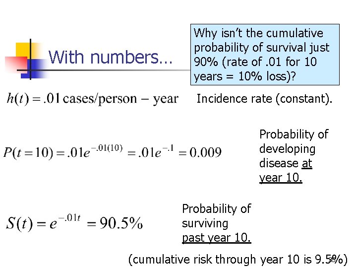
With numbers… Why isn’t the cumulative probability of survival just 90% (rate of. 01 for 10 years = 10% loss)? Incidence rate (constant). Probability of developing disease at year 10. Probability of surviving past year 10. 38 (cumulative risk through year 10 is 9. 5%)

Example… Recall this graphic. Does it look Normal, Weibull, exponential? 39

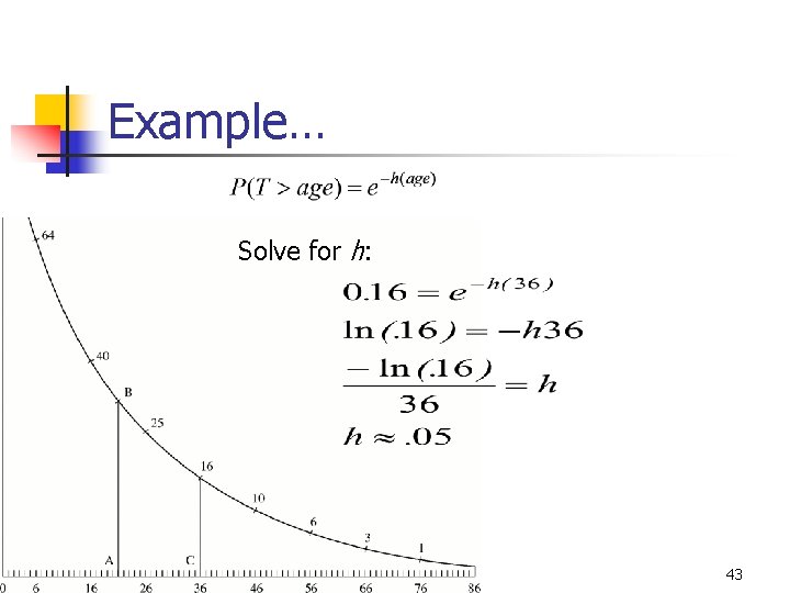
Example… One way to describe the survival distribution here is: P(T>76)=. 01 P(T>36) =. 16 P(T>20)=. 20, etc. 40

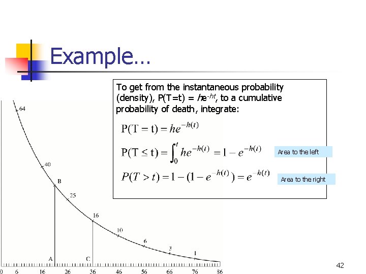
Example… Or, more compactly, try to describe this as an exponential probability function—since that is how it is drawn! Recall the exponential probability distribution: If T ~ exp (h), then P(T=t) = he-ht Where h is a constant rate. Here: Event time, T ~ exp (Rate) 41

Example… To get from the instantaneous probability (density), P(T=t) = he-ht, to a cumulative probability of death, integrate: Area to the left Area to the right 42

Example… Solve for h: 43

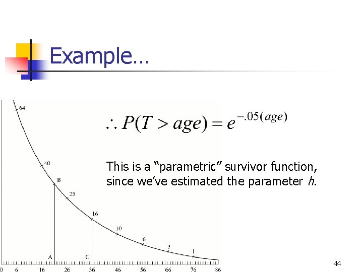
Example… This is a “parametric” survivor function, since we’ve estimated the parameter h. 44

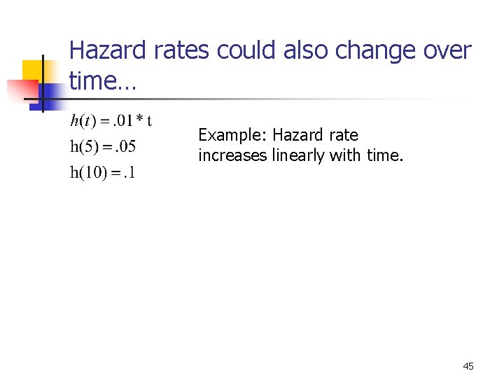
Hazard rates could also change over time… Example: Hazard rate increases linearly with time. 45

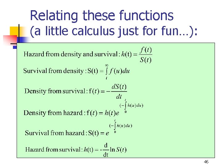
Relating these functions (a little calculus just for fun…): 46

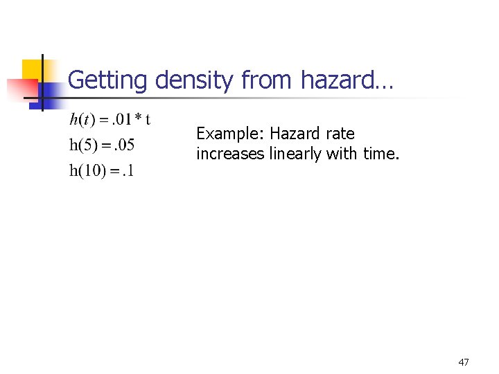
Getting density from hazard… Example: Hazard rate increases linearly with time. 47

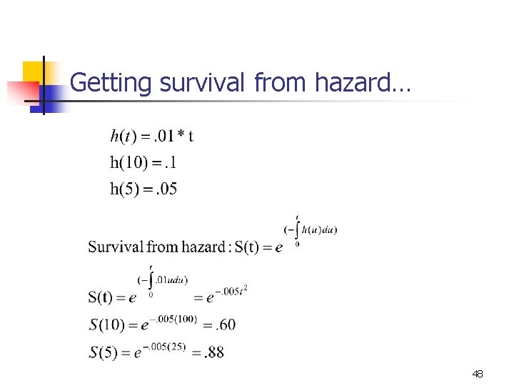
Getting survival from hazard… 48

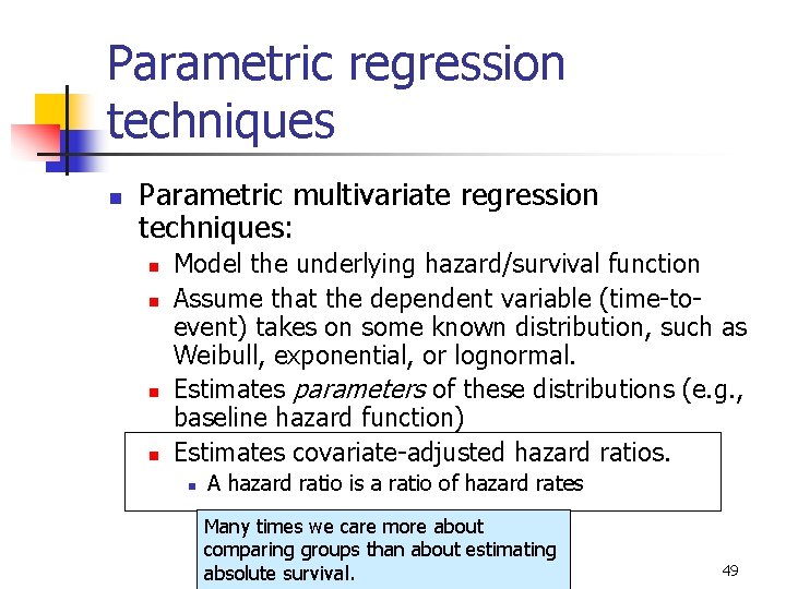
Parametric regression techniques n Parametric multivariate regression techniques: n n Model the underlying hazard/survival function Assume that the dependent variable (time-toevent) takes on some known distribution, such as Weibull, exponential, or lognormal. Estimates parameters of these distributions (e. g. , baseline hazard function) Estimates covariate-adjusted hazard ratios. n A hazard ratio is a ratio of hazard rates Many times we care more about comparing groups than about estimating absolute survival. 49

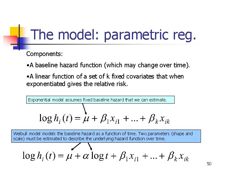
The model: parametric reg. Components: • A baseline hazard function (which may change over time). • A linear function of a set of k fixed covariates that when exponentiated gives the relative risk. Exponential model assumes fixed baseline hazard that we can estimate. Weibull models the baseline hazard as a function of time. Two parameters (shape and scale) must be estimated to describe the underlying hazard function over time. 50

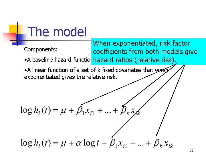
The model When exponentiated, risk factor Components: coefficients from both models give • A baseline hazard functionhazard ratios (relative risk). • A linear function of a set of k fixed covariates that when exponentiated gives the relative risk. 51

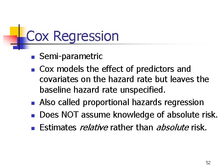
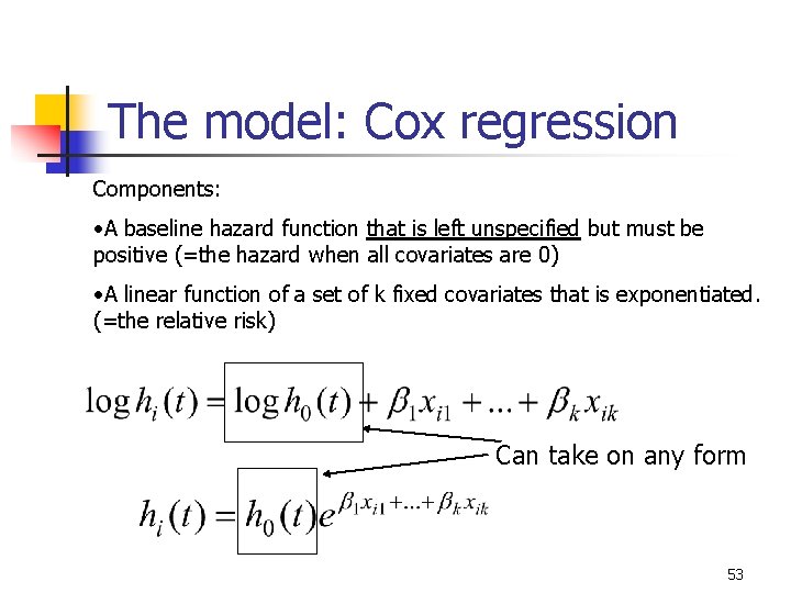
Cox Regression n n Semi-parametric Cox models the effect of predictors and covariates on the hazard rate but leaves the baseline hazard rate unspecified. Also called proportional hazards regression Does NOT assume knowledge of absolute risk. Estimates relative rather than absolute risk. 52

The model: Cox regression Components: • A baseline hazard function that is left unspecified but must be positive (=the hazard when all covariates are 0) • A linear function of a set of k fixed covariates that is exponentiated. (=the relative risk) Can take on any form 53

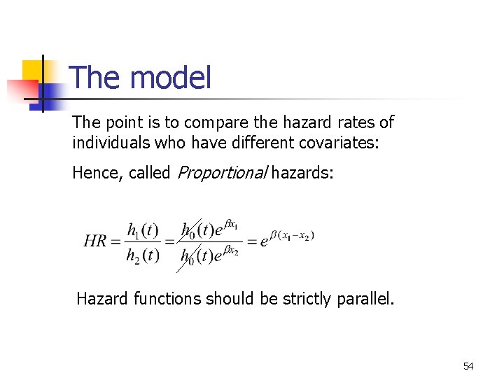
The model The point is to compare the hazard rates of individuals who have different covariates: Hence, called Proportional hazards: Hazard functions should be strictly parallel. 54

Introduction to Kaplan-Meier Non-parametric estimate of the survival function: No math assumptions! (either about the underlying hazard function or about proportional hazards). Simply, the empirical probability of surviving past certain times in the sample (taking into account censoring). 55

Introduction to Kaplan-Meier n n Non-parametric estimate of the survival function. Commonly used to describe survivorship of study population/s. Commonly used to compare two study populations. Intuitive graphical presentation. 56

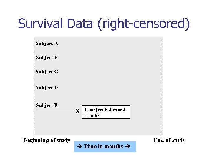
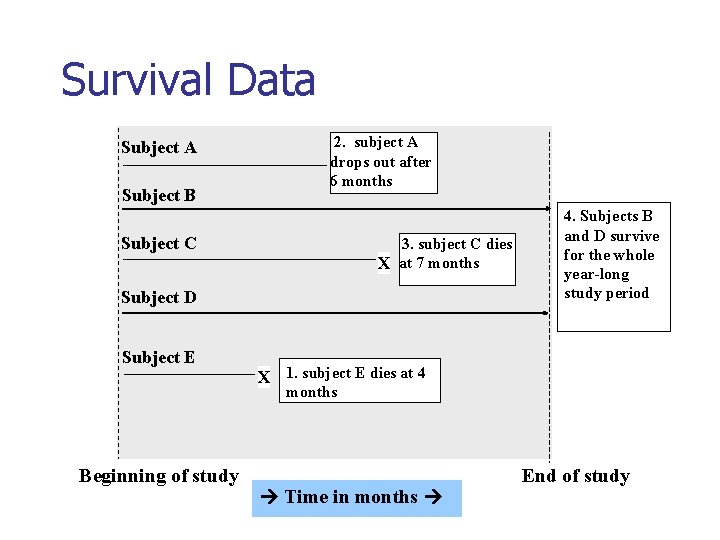
Survival Data (right-censored) Subject A Subject B Subject C Subject D Subject E X 1. subject E dies at 4 months Beginning of study Time in months End of study

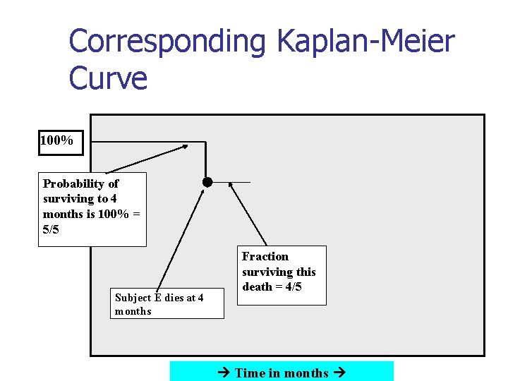
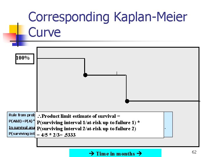
Corresponding Kaplan-Meier Curve 100% Probability of surviving to 4 months is 100% = 5/5 Subject E dies at 4 months Fraction surviving this death = 4/5 Time in months

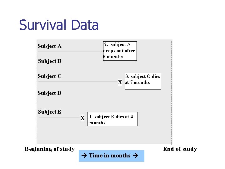
Survival Data Subject A Subject B 2. subject A drops out after 6 months Subject C 3. subject C dies X at 7 months Subject D Subject E X 1. subject E dies at 4 months Beginning of study Time in months End of study

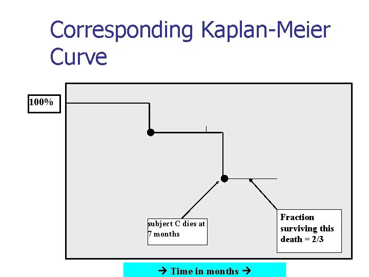
Corresponding Kaplan-Meier Curve 100% subject C dies at 7 months Time in months Fraction surviving this death = 2/3

Survival Data Subject A Subject B 2. subject A drops out after 6 months Subject C 3. subject C dies X at 7 months Subject D Subject E 4. Subjects B and D survive for the whole year long study period X 1. subject E dies at 4 months Beginning of study Time in months End of study

Corresponding Kaplan-Meier Curve 100% Rule from probability theory: limit Product estimate of survival = P(A&B)=P(A)*P(B) if A and B independent P(surviving interval 1/at risk up to failure 1) * In survival analysis: intervals are defined by failures (2 leading P(surviving interval 2/at risk upintervals to failure 2) to failures here). P(surviving intervals 2)=P(surviving interval 1)*P(surviving interval 2) = 4/51 *and 2/3=. 5333 Time in months 62

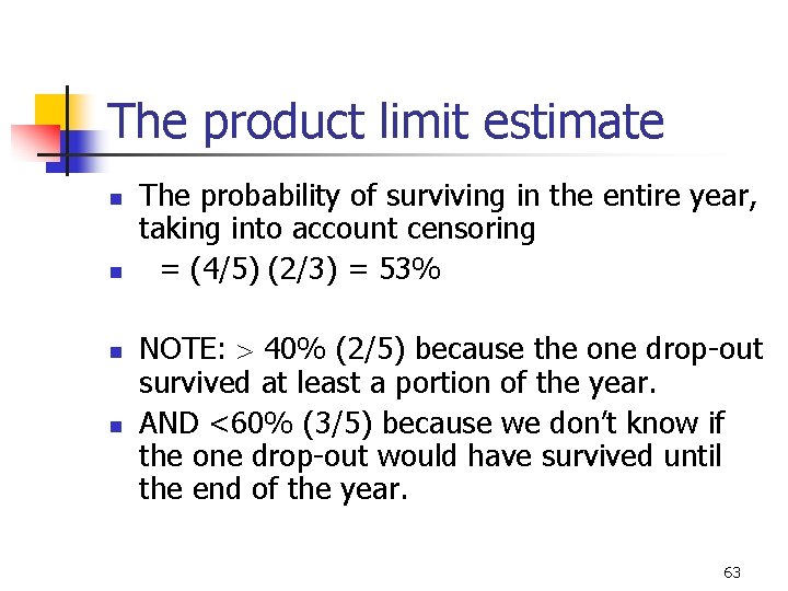
The product limit estimate n n The probability of surviving in the entire year, taking into account censoring = (4/5) (2/3) = 53% NOTE: 40% (2/5) because the one drop-out survived at least a portion of the year. AND <60% (3/5) because we don’t know if the one drop-out would have survived until the end of the year. 63

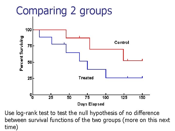
Comparing 2 groups Use log-rank test to test the null hypothesis of no difference between survival functions of the two groups (more on this next time)

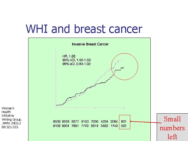
Caveats n Survival estimates can be unreliable toward the end of a study when there are small numbers of subjects at risk of having an event. 65

WHI and breast cancer Women’s Health Initiative Writing Group. JAMA. 2002; 2 88: 321 -333. Small numbers left

Limitations of Kaplan-Meier • • Mainly descriptive Doesn’t control for covariates Requires categorical predictors Can’t accommodate time-dependent variables 67

All about Kaplan-Meier next lecture… 68

Overview of SAS PROCS n n n LIFETEST - Produces life tables and Kaplan-Meier survival curves. Is primarily for univariate analysis of the timing of events. LIFEREG – Estimates regression models with censored, continuous-time data under several alternative distributional assumptions. Does not allow for time-dependent covariates. PHREG– Uses Cox’s partial likelihood method to estimate regression models with censored data. Handles both continuous-time and discrete-time data and allows for time-dependent covariables 69

References Paul Allison. Survival Analysis Using SAS Institute Inc. , Cary, NC: 2003. 70