Survival Analysis Diane Stockton Survival Curves A survival

Survival Analysis Diane Stockton

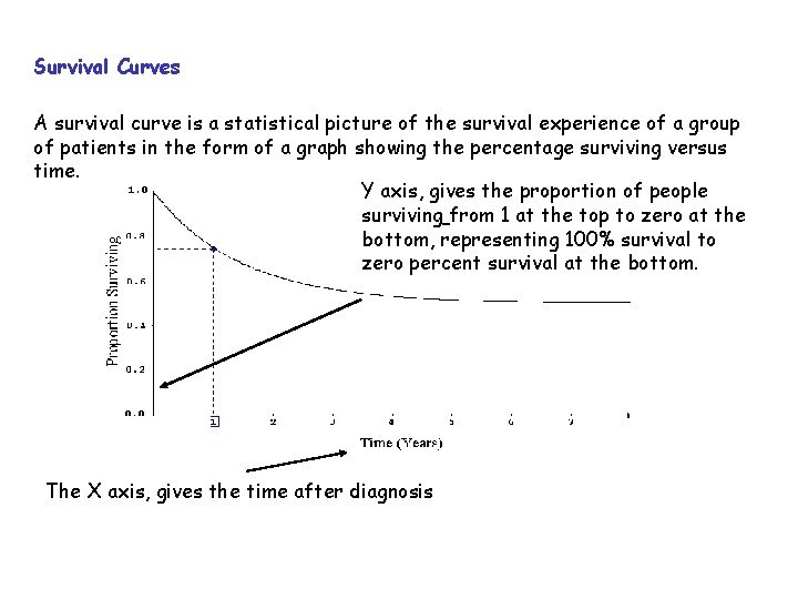
Survival Curves A survival curve is a statistical picture of the survival experience of a group of patients in the form of a graph showing the percentage surviving versus time. Y axis, gives the proportion of people surviving from 1 at the top to zero at the bottom, representing 100% survival to zero percent survival at the bottom. The X axis, gives the time after diagnosis

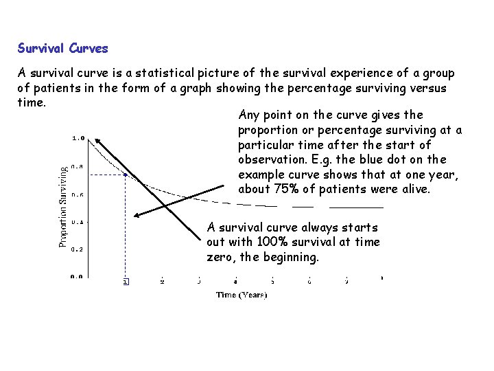
Survival Curves A survival curve is a statistical picture of the survival experience of a group of patients in the form of a graph showing the percentage surviving versus time. Any point on the curve gives the proportion or percentage surviving at a particular time after the start of observation. E. g. the blue dot on the example curve shows that at one year, about 75% of patients were alive. A survival curve always starts out with 100% survival at time zero, the beginning.

Questions in survival analyses Which Survival? • Observed (or crude) survival • Cause-specific (also known as Net or Corrected) survival • Relative survival • Period survival Data issues • Censoring • Life tables • Standardisation Modelling survival

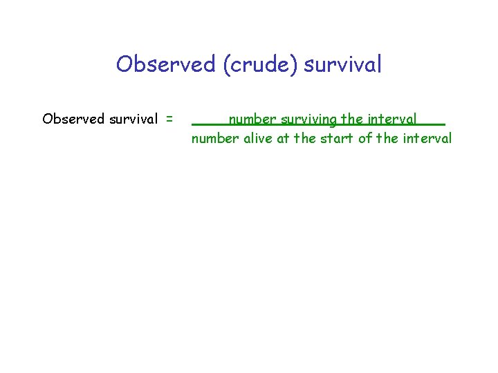
Observed (crude) survival Observed survival = number surviving the interval number alive at the start of the interval

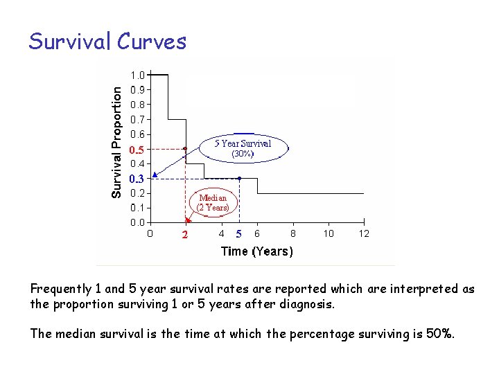
Survival Curves Frequently 1 and 5 year survival rates are reported which are interpreted as the proportion surviving 1 or 5 years after diagnosis. The median survival is the time at which the percentage surviving is 50%.

Survival Curves • The experience of a particular group as represented by a staircase curve can be considered an estimate or sample of what the "real" survival curve is for all people with the same circumstances. • As with other estimates, the accuracy improves as the sample size increases. • With staircase curves, as the group of patients is larger, the step down caused by each death is smaller. • If the times of the deaths are plotted accurately, then you can see that as the size of the group increases the staircase will become closer and closer to the ideal of a smooth curve.

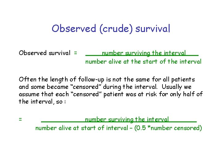
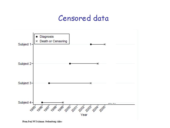
Observed (crude) survival Observed survival = number surviving the interval number alive at the start of the interval Often the length of follow-up is not the same for all patients and some became “censored” during the interval. Usually we assume that each “censored” patient was at risk for only half of the interval, so : = number surviving the interval number alive at start of interval – (0. 5 *number censored)

Censored data From Paul W Dickman Gothenburg slides

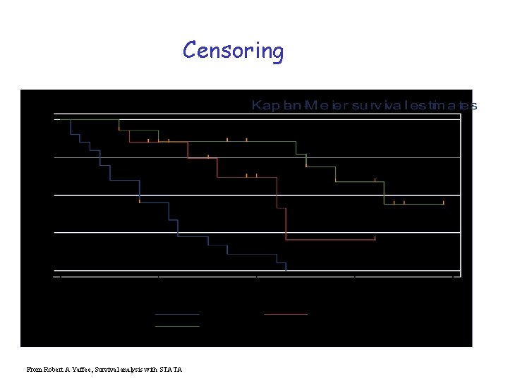
Censoring • When a patient is censored the curve doesn't take a step down as it does when a patient dies. • But censoring the patient reduces the number of patients who are contributing to the curve, so each death after that point represents a higher proportion of the remaining population, and so every step down afterwards will be a little bit larger than it would have been.

Censoring From Robert A Yaffee, Survival analysis with STATA

Cause-specific (or net or corrected) Survival Cause of death from the death certificate is used to attribute the death to • the disease of interest • other causes BUT……. . Which deaths should be considered attributable to the disease of interest? Are the death certificates available and accurate? The analysis is exactly the same as for observed survival (actuarial or Kaplan-meier) but those dying from other causes are counted as censored at their time of death

Censoring From Robert A Yaffee, Survival analysis with STATA

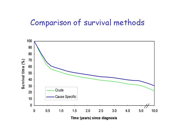
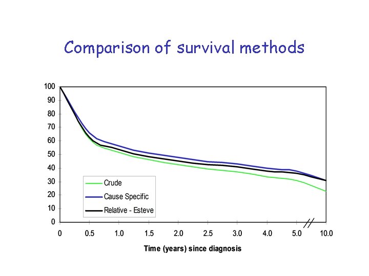
Comparison of survival methods

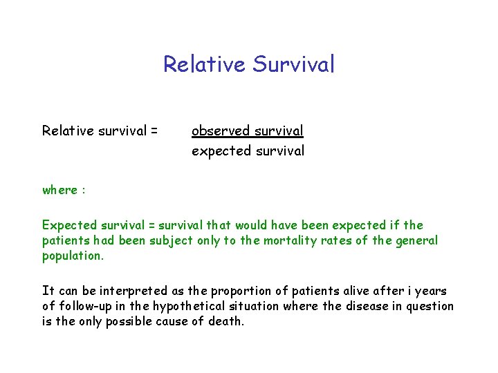
Relative Survival Relative survival = observed survival expected survival where : Expected survival = survival that would have been expected if the patients had been subject only to the mortality rates of the general population. It can be interpreted as the proportion of patients alive after i years of follow-up in the hypothetical situation where the disease in question is the only possible cause of death.

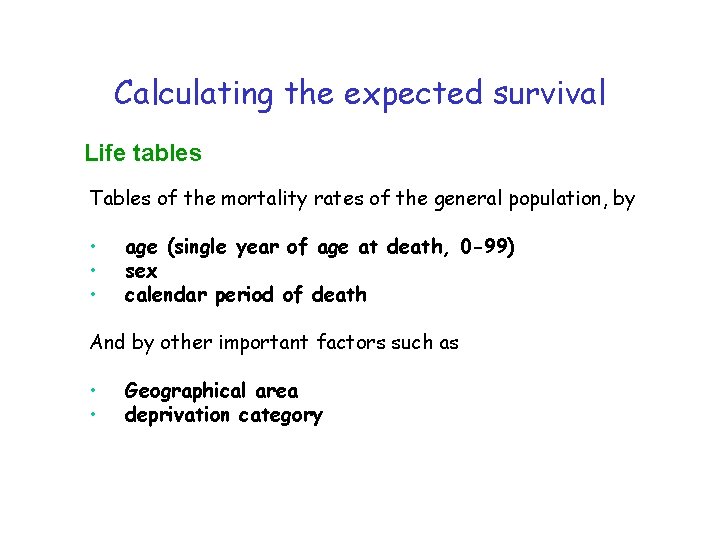
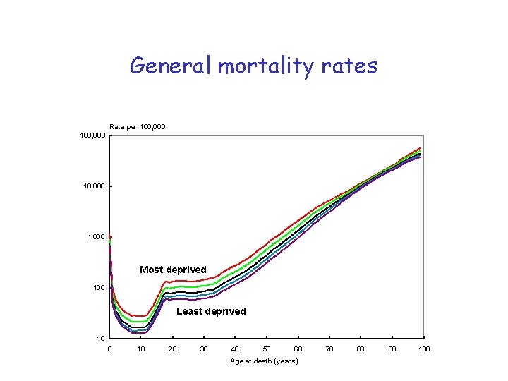
Calculating the expected survival Life tables Tables of the mortality rates of the general population, by • • • age (single year of age at death, 0 -99) sex calendar period of death And by other important factors such as • • Geographical area deprivation category

General mortality rates Rate per 100, 000 10, 000 1, 000 Most deprived 100 Least deprived 10 0 10 20 30 40 50 60 Age at death (years) 70 80 90 100

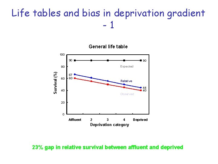
Life tables and bias in deprivation gradient -1 General life table 100 90 90 Expected Survival (%) 80 60 67 60 Relative 44 40 40 Observed 20 0 Affluent 2 3 4 Deprived Deprivation category 23% gap in relative survival between affluent and deprived

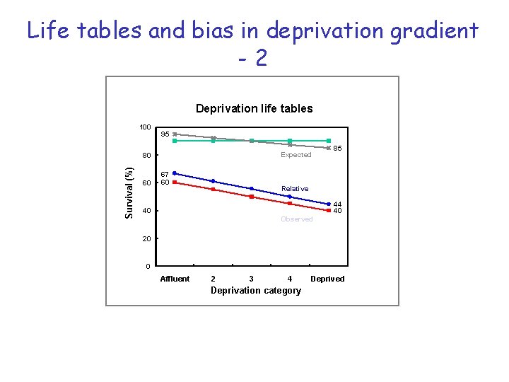
Life tables and bias in deprivation gradient -2 Deprivation life tables 100 95 Expected Survival (%) 80 60 67 60 85 Relative 44 40 40 Observed 20 0 Affluent 2 3 4 Deprivation category Deprived

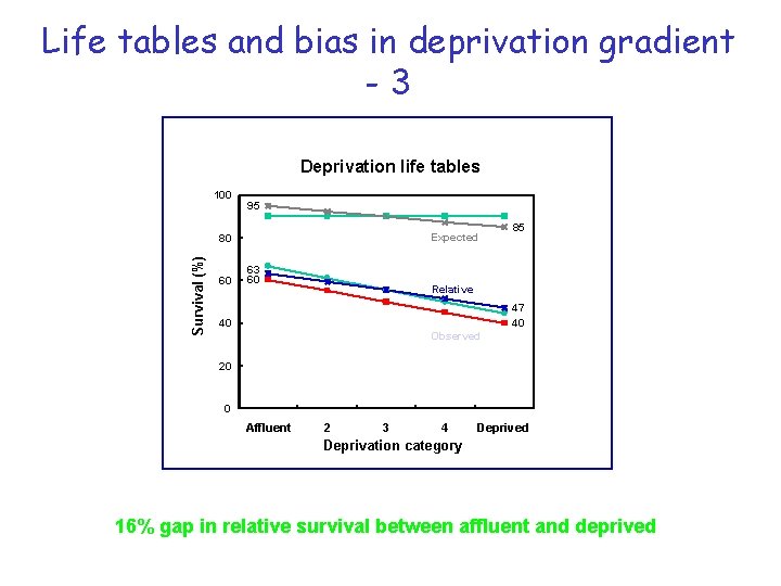
Life tables and bias in deprivation gradient -3 Deprivation life tables 100 95 Expected Survival (%) 80 60 63 60 85 Relative 47 40 40 Observed 20 0 Affluent 2 3 4 Deprived Deprivation category 16% gap in relative survival between affluent and deprived

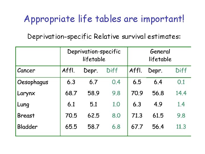
Life Tables The use of the same life table for groups for whom general mortality is known to differ can lead to bias because the expected survival will be under estimated for the groups who have better than average survival and hence the relative survival will be over estimated and visa versa for the groups who have worse than average survival

Appropriate life tables are important! Deprivation-specific Relative survival estimates:

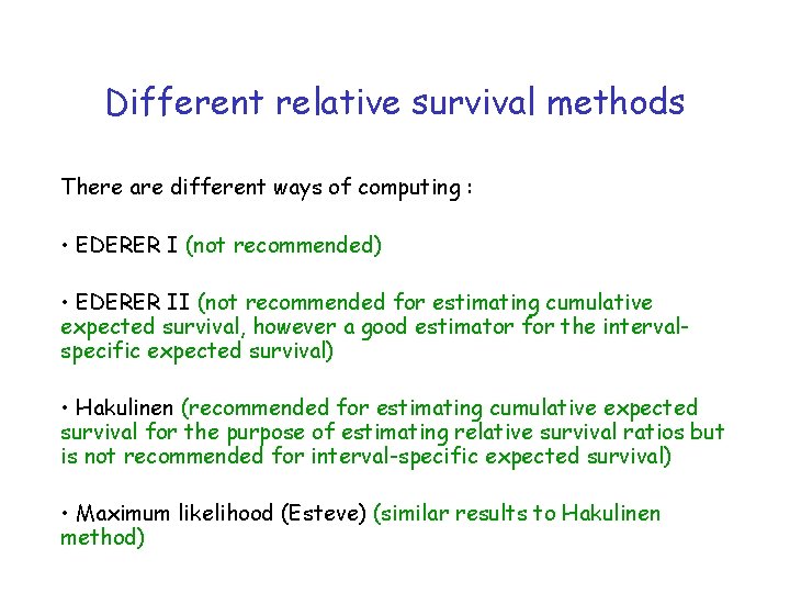
Different relative survival methods There are different ways of computing : • EDERER I (not recommended) • EDERER II (not recommended for estimating cumulative expected survival, however a good estimator for the intervalspecific expected survival) • Hakulinen (recommended for estimating cumulative expected survival for the purpose of estimating relative survival ratios but is not recommended for interval-specific expected survival) • Maximum likelihood (Esteve) (similar results to Hakulinen method)

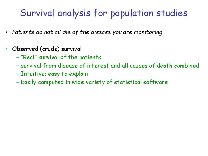
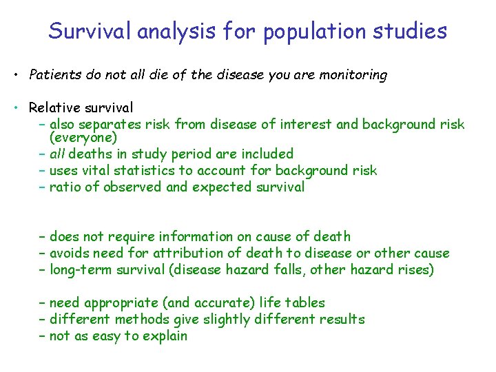
Survival analysis for population studies • Patients do not all die of the disease you are monitoring • Observed (crude) survival – “Real” survival of the patients – survival from disease of interest and all causes of death combined – Intuitive; easy to explain – Easily computed in wide variety of statistical software

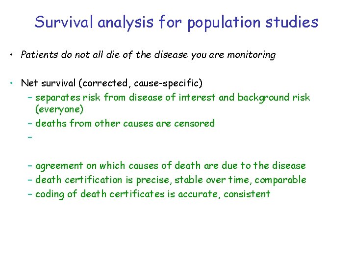
Survival analysis for population studies • Patients do not all die of the disease you are monitoring • Net survival (corrected, cause-specific) – separates risk from disease of interest and background risk (everyone) – deaths from other causes are censored – survival from cancer in the absence of other causes – agreement on which causes of death are due to the disease – death certification is precise, stable over time, comparable – coding of death certificates is accurate, consistent

Survival analysis for population studies • Patients do not all die of the disease you are monitoring • Relative survival – also separates risk from disease of interest and background risk (everyone) – all deaths in study period are included – uses vital statistics to account for background risk – ratio of observed and expected survival – survival relative to that of general population – does not require information on cause of death – avoids need for attribution of death to disease or other cause – long-term survival (disease hazard falls, other hazard rises) – need appropriate (and accurate) life tables – different methods give slightly different results – not as easy to explain

Comparison of survival methods

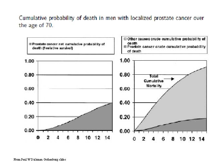
From Paul W Dickman Gothenburg slides

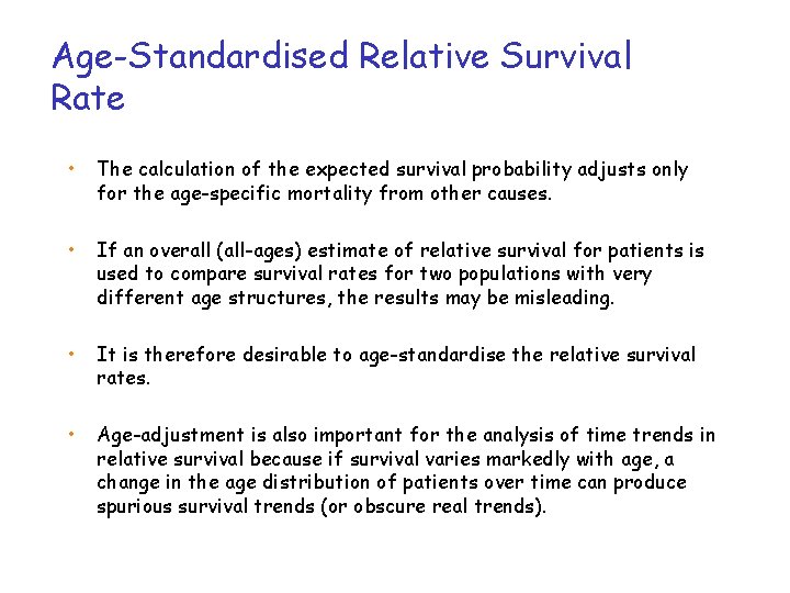
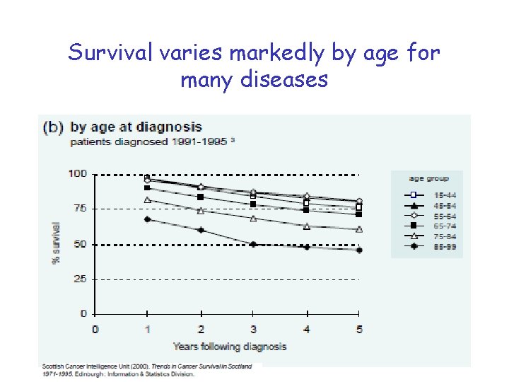
Age-Standardised Relative Survival Rate • The calculation of the expected survival probability adjusts only for the age-specific mortality from other causes. • If an overall (all-ages) estimate of relative survival for patients is used to compare survival rates for two populations with very different age structures, the results may be misleading. • It is therefore desirable to age-standardise the relative survival rates. • Age-adjustment is also important for the analysis of time trends in relative survival because if survival varies markedly with age, a change in the age distribution of patients over time can produce spurious survival trends (or obscure real trends).

Survival varies markedly by age for many diseases

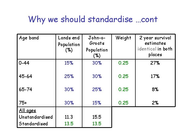
Why we should standardise …cont Age band Lands end Population (%) John-o. Groats Population (%) Weight 2 year survival estimates identical in both places 0 -44 15% 30% 0. 25 27% 45 -64 25% 30% 0. 25 17% 65 -74 30% 25% 0. 25 8% 75+ 30% 15% 0. 25 2% All ages Unstandardised Standardised 11. 3 13. 5 15. 5 13. 5

Age-standardisation Advantages None of the routine survival methods adjust for age or sex (not even relative survival) • Standardising allows comparison with other populations or over time when the population structures are not the same … the other option is modelling which is discussed later

Age-standardisation Limitations • No routinely-used common standard population for survival analyses – create a standard that is sensible for your data • Unclear what to do when there is no survival estimate for an age-group • Obviously more time consuming than “all ages” estimates

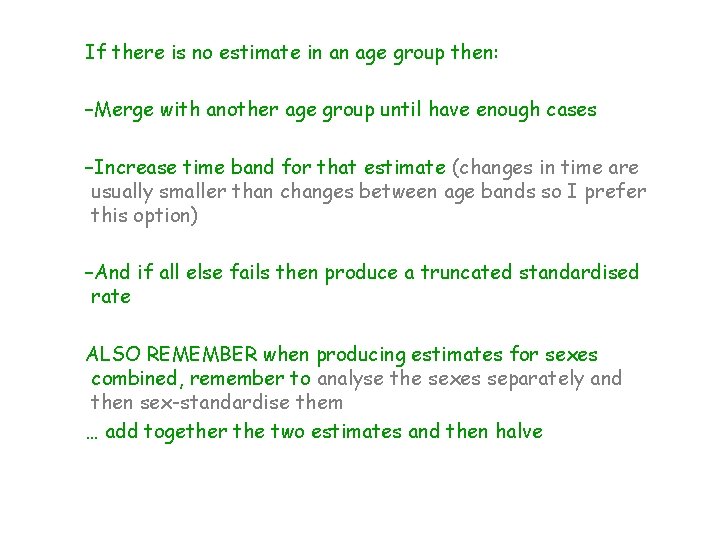
If there is no estimate in an age group then: –Merge with another age group until have enough cases –Increase time band for that estimate (changes in time are usually smaller than changes between age bands so I prefer this option) –And if all else fails then produce a truncated standardised rate ALSO REMEMBER when producing estimates for sexes combined, remember to analyse the sexes separately and then sex-standardise them … add together the two estimates and then halve

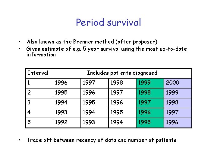
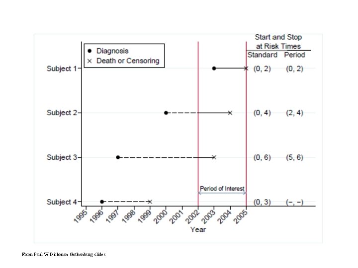
Period survival • • Also known as the Brenner method (after proposer) Gives estimate of e. g. 5 year survival using the most up-to-date information Interval • Includes patients diagnosed 1 1996 1997 1998 1999 2000 2 1995 1996 1997 1998 1999 3 1994 1995 1996 1997 1998 4 1993 1994 1995 1996 1997 5 1992 1993 1994 1995 1996 Trade off between recency of data and number of patients

From Paul W Dickman Gothenburg slides

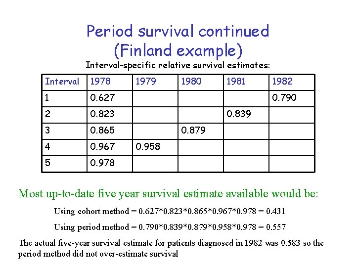
Period survival continued (Finland example) Interval-specific relative survival estimates: Interval 1978 1 0. 627 2 0. 823 3 0. 865 4 0. 967 5 0. 978 1979 1980 1981 1982 0. 790 0. 839 0. 879 0. 958 Most up-to-date five year survival estimate available would be: Using cohort method = 0. 627*0. 823*0. 865*0. 967*0. 978 = 0. 431 Using period method = 0. 790*0. 839*0. 879*0. 958*0. 978 = 0. 557 The actual five-year survival estimate for patients diagnosed in 1982 was 0. 583 so the period method did not over-estimate survival

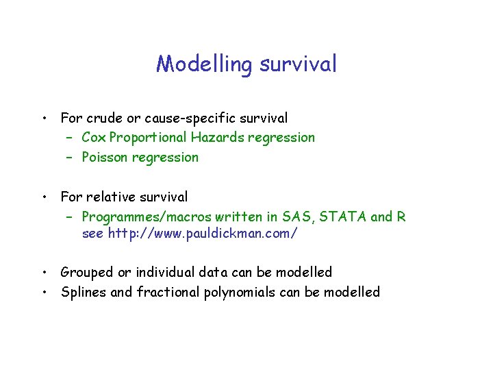
Modelling survival • For crude or cause-specific survival – Cox Proportional Hazards regression – Poisson regression • For relative survival – Programmes/macros written in SAS, STATA and R see http: //www. pauldickman. com/ • Grouped or individual data can be modelled • Splines and fractional polynomials can be modelled

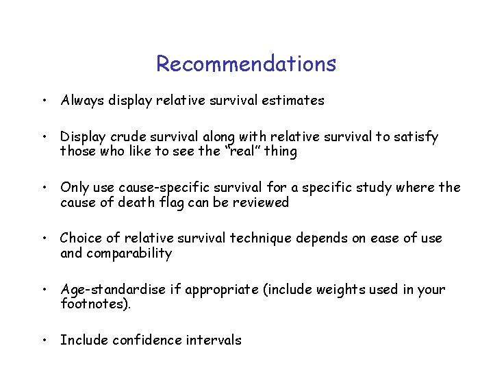
Recommendations • Always display relative survival estimates • Display crude survival along with relative survival to satisfy those who like to see the “real” thing • Only use cause-specific survival for a specific study where the cause of death flag can be reviewed • Choice of relative survival technique depends on ease of use and comparability • Age-standardise if appropriate (include weights used in your footnotes). • Include confidence intervals

Useful links / contacts • Presentations, statistical programme code, scientific papers and examples of survival analyses http: //www. pauldickman. com/ • STATA ado files for the maximum likelihood relative survival method http: //www. lshtm. ac. uk/eph/ncde/cancersurvival/tools/ My details: diane. stockton@nhs. net 0131 275 6817