4 Survival Analysis Notes based on Klein J

Διάλεξη 4. Survival Analysis Notes based on Klein J. P. and Moeschberger M. L. , Survival Analysis- Techniques for Censored and Truncated Data, Series: Statistics for Biology and Health, Springer 2003.

1. Introduction: --Survival analysis: analysis for cohort studies; an alternative approach to the analysis using rate ratios. --Studies “time to an event” instead of the rate of the event in the population The analysis of rates assumes that the rate(s) vary only gradually with time or age. This assumption is plausible only if the events/diseases are relatively rare. These methods are less appropriate when: 1) The incidence rates vary rapidly over time/age; 2) Many of the individuals experience the event, and interest lies on the time elapsed from entry to the event In such cases it is better to use survival analysis. Examples: time to death following the diagnosis of breast cancer. Time to remission of disease following treatment. We define as survival data or failure time data the data from a cohort study where the time to the event is the main outcome of interest. Note that the event of interest is not necessarily “bad-failure” e. g. time to a pregnancy. Survival time for each subject is the time from a predetermined starting point to the occurrence of the event of interest. Emphasis should be put on the definition of the starting point. E. g. entry to the study; onset of disease; start of treatment.

Survival outcome: Time to event and event In survival we have a two-variable outcome for each individual i: • Time variable: ti = time at last disease-free observation or time at event – Failure time random variables are always nonnegative. That is, if we denote the failure time by T, then T ≥ 0. • Event variable: δi =1 if had the event; δi =0 no event by time ti – If δi=0 then the observation is censored

Time-to-event random variable In order to define a time to event (or failure time) random variable, we need at least: 1. an unambiguous time origin (e. g. randomization to clinical trial, surgery, disease diagnosis) 2. a time scale (e. g. real time (days, years)) 3. definition of the event (e. g. death, childbirth, graduation)

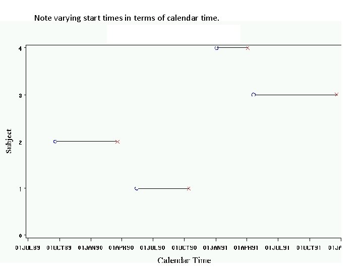
Note varying start times in terms of calendar time.

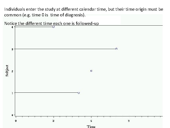
Individuals enter the study at different calendar time, but their time origin must be common (e. g. time 0 is time of diagnosis). Notice the different time each one is followed-up

Censoring and Truncation • Censoring occurs when some lifetimes are known to have occurred only within a certain interval- exact lifetimes are not known for some individuals in a study • Truncation occurs when subjects come under observation only if their failure times lie within a specific interval – A truncated observation is one which is unobservable due to a selection process inherent in the study design.

Typical Censoring Mechanisms • Right censoring – Type II censoring – Random censoring • Left censoring • Double censoring (a data set containing left & right censoring data) • Interval censoring

Right Censoring • Observation begins at the defined time origin and ceases before the event of interest is realized. – The survival time is only known to exceed a certain value. – Incomplete nature of the observation occurs in the right tail of the time axis.

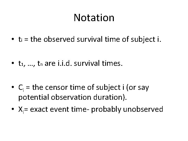
Notation • ti = the observed survival time of subject i. • t 1, …, tn are i. i. d. survival times. • Ci = the censor time of subject i (or say potential observation duration). • Xi= exact event time- probably unobserved

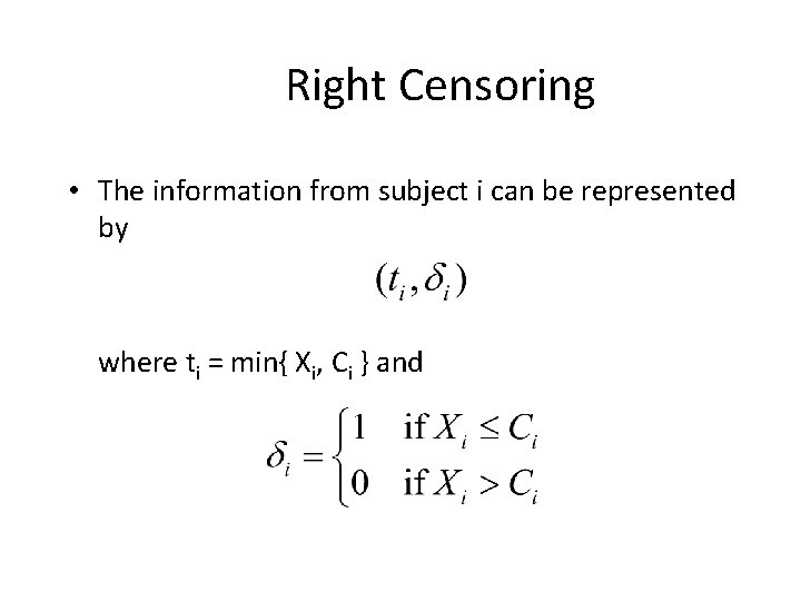
Right Censoring • The information from subject i can be represented by where ti = min{ Xi, Ci } and

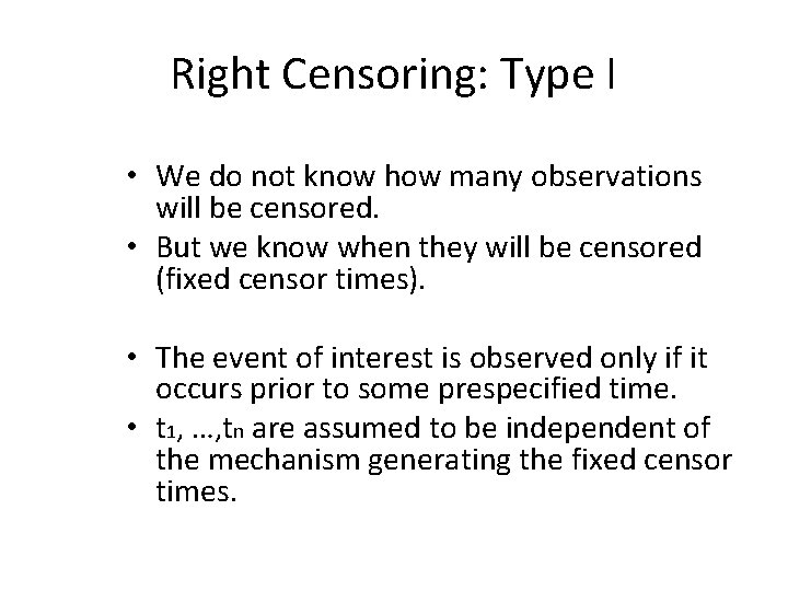
Right Censoring: Type I • We do not know how many observations will be censored. • But we know when they will be censored (fixed censor times). • The event of interest is observed only if it occurs prior to some prespecified time. • t 1, …, tn are assumed to be independent of the mechanism generating the fixed censor times.

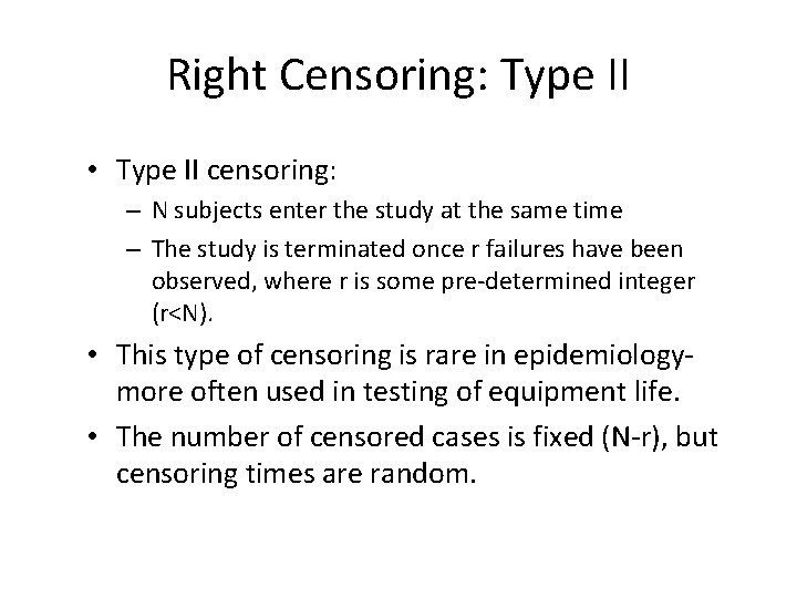
Right Censoring: Type II • Type II censoring: – N subjects enter the study at the same time – The study is terminated once r failures have been observed, where r is some pre-determined integer (r<N). • This type of censoring is rare in epidemiologymore often used in testing of equipment life. • The number of censored cases is fixed (N-r), but censoring times are random.

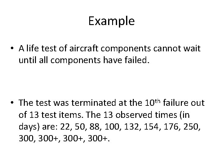
Example • A life test of aircraft components cannot wait until all components have failed. • The test was terminated at the 10 th failure out of 13 test items. The 13 observed times (in days) are: 22, 50, 88, 100, 132, 154, 176, 250, 300, 300+, 300+.

Right Censoring: Random • Arises when other competing events cause subjects to be removed from the study. • The censor times are random and the number of censored cases is also random.

Right Censoring: Random • Some events which cause the subject to be randomly censored, with respect to the event of interest, include – Patient withdrawal from a clinical trial – Competing event – Migration/ move to other city

Example- the Trinidad dataset • This is a 10 -year follow-up cohort study. During this time dates and causes of death of those who died were recorded. • The event of interest was death from cardiovascular disease. • Individuals alive at the end of the 10 -year follow-up were considered censored (i. e. that they have experience the event of interest at 10+ years).

Example- the Trinidad dataset • We will use a subset of this cohort consisting of 318 men who were over 60 years old at the time of the survey. • 109 men described themselves as ‘current smokers’ while 208 as non or ex smokers. • There were 88 deaths recorded in this group from any cause and this is what we will use as the event of interest.

2. 1 The Lifetable method the Trinidad dataset • Divide the period of observation into a series of time intervals and estimate the conditional (interval-specific) survival proportion for each interval. • The cumulative survivor function, S(x), at the end of a specified interval is given by the product of the intervalspecific survival proportions for all intervals up to and including the specified interval. • In the absence of censoring, the interval-specific survivor proportion is p=(l-d)/l, where d is the number of events (deaths) observed during the interval and l is the number of patients alive at the start of the interval.

2. 1 The Lifetable Method (cont. ) § § § In the presence of censoring, it is assumed that censoring occurs uniformly throughout the interval such that each individual with a censored survival time is at risk for, on average, half the interval. The effective number of patients at risk during the interval is given by l*=l-(w/2) where l is the number of patients alive at the start of the interval and w is the number of censorings during the interval. The estimated interval-specific survival proportion is then given by p=(l*-d)/l*.

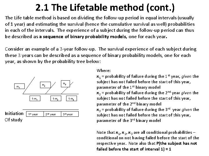
2. 1 The Lifetable method (cont. ) The Life table method is based on dividing the follow-up period in equal intervals (usually of 1 year) and estimating the survival (hence the cumulative survival as well) probabilities in each of the intervals. The experience of a subject during the follow-up period can thus be described as a sequence of binary probability models, one for each year. Consider an example of a 3 -year follow-up. The survival experience of each subject during these 3 years can be described as a sequence of binary probability models, one for each year, as shown by the probability tree below: 1 -π1 Initiation Of study π3 π2 π1 1 st year 1 -π2 2 nd year 1 -π3 3 rd year Where: π1 = probability of failure during the 1 st year, given the subject has not failed before the start of this year, parameter of the 1 st binary model π2 = probability of failure during the 2 nd year given the subject has not failed before the start of this year, parameter of the 2 nd binary model π3 = probability of failure during the 3 rd year given the subject has not failed before the start of this year, parameter of the 3 rd binary model Note that π1, π2, π3 are all conditional probabilities – conditional on not having failed before the start of the respective year. Note also that P(the subject has not failed before the start of interval 1) = 1

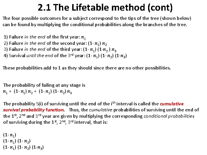
2. 1 The Lifetable method (cont) The four possible outcomes for a subject correspond to the tips of the tree (shown below) can be found by multiplying the conditional probabilities along the branches of the tree. 1) Failure in the end of the first year: π1 2) Failure in the end of the second year: (1 - π1) π2 3) Failure in the end of the third year: (1 - π1) (1 -π2 ) π3 4) Survival until the end of the 3 rd year: (1 - π1) (1 - π 2) (1 -π3) These probabilities add to 1 as they should since there are no other possibilities. The probability of failing at any stage is π1 + (1 - π1) π2 + (1 - π1) (1 - π2) π3 The probability S(i) of surviving until the end of the ith interval is called the cumulative survival probability function. Thus, the cumulative probabilities of surviving until the end of the 1 st, 2 nd and 3 rd year are given by multiplying the corresponding conditional probabilities of surviving during the 1 st, 2 nd, 3 rd interval, that is: (1 - π1) (1 - π2) (1 -π3)

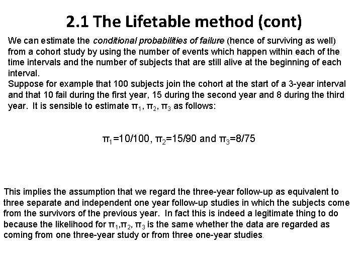
2. 1 The Lifetable method (cont) We can estimate the conditional probabilities of failure (hence of surviving as well) from a cohort study by using the number of events which happen within each of the time intervals and the number of subjects that are still alive at the beginning of each interval. Suppose for example that 100 subjects join the cohort at the start of a 3 -year interval and that 10 fail during the first year, 15 during the second year and 8 during the third year. It is sensible to estimate π1, π2, π3 as follows: π1=10/100, π2=15/90 and π3=8/75 This implies the assumption that we regard the three-year follow-up as equivalent to three separate and independent one year follow-up studies in which the subjects come from the survivors of the previous year. In fact this is indeed a legitimate thing to do because the likelihood for π1, π2, π3 is the same whether the data are regarded as coming from one three-year study or from three one-year studies.

Proof: (Clayton and Hills, page 31) The probabilities of the four possible outcomes in the three-year study are: π1 (1 - π1) π2 (1 - π1) (1 -π2 ) π3 (1 - π1) (1 - π2) (1 -π3) A subject who fails during the first year therefore contributes: log(π1) to the log likelihood. A subject who fails during the second year contributes: log (1 - π1) + log (π2 ) and a subject who fails during the third year contributes: log (1 - π1) + log (1 - π2 ) + log(π3). A subject who survives all three years contributes: log (1 - π1) + log (1 - π2 ) + log (1 - π3) Multiplying these by the numbers of subjects with each outcome, that is in our example 10, 15, 8, and 67 respectively, and adding, gives a total log likelihood of: 10 log(π1)+ 90 log (1 - π1) + 15 log (π2 ) + 75 log (1 - π2) + 8 log(π3 ) + 67 log (1 - π3 ). This is the same as the log likelihood obtained by regarding the data as from three separate and independent one-year studies; the first based on 10 failures and 90 survivors, the second on 15 failures and 75 survivors, and the third on 8 failures and 67 survivors.

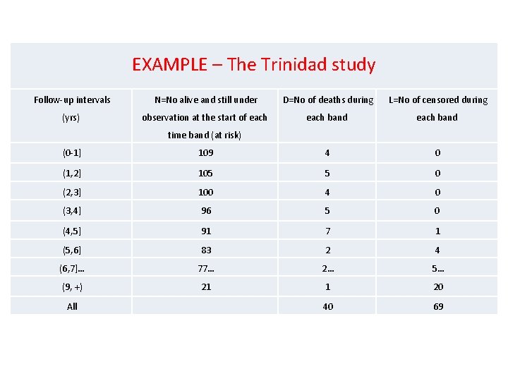
EXAMPLE – The Trinidad study Follow-up intervals N=No alive and still under D=No of deaths during L=No of censored during (yrs) observation at the start of each band 4 0 time band (at risk) (0 -1] 109 (1, 2] 105 5 0 (2, 3] 100 4 0 (3, 4] 96 5 0 (4, 5] 91 7 1 (5, 6] 83 2 4 (6, 7]… 77… 2… 5… (9, +) 21 1 20 All 40 69

ESTIMATION - EXAMPLE 4 5 4 0 0 0 109 105 (0 -1] (1 -2] 100 (2 -3] 96 According to what we have said so far the conditional probability of death from any cause within any interval i will be estimated as the ratio between the number of failures (Di) that occurred within the ith interval and the number of subjects still alive at the beginning of the ith interval (subjects at risk, Ni). For example the probability of death in the second year given that a person survived during the first year is 5/105=0. 04762. Prob(death in interval i | survival up to i) = Number of deaths in i Number at risk in the beginning of i However this is relevant only if there are no censored observations within interval i. If censored observations exist they complicate the situation because we do not know at what precise time the censored observation stopped being at risk. The accepted method is to assume that censored observations are, on average, at risk for half the follow-up interval and to adjust the denominator of the probability of death calculation for the particular interval accordingly: Prob(death in interval i | survival up to i) = Number of deaths in i / {(number at risk in i) - (0. 5 x Number Censored)}

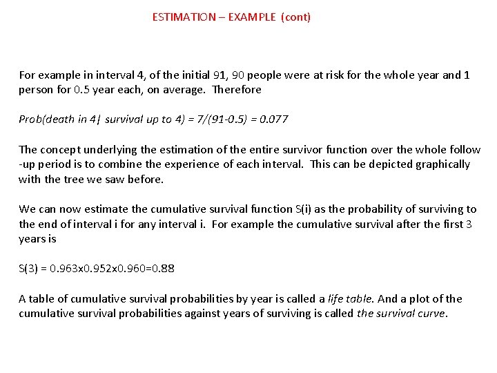
ESTIMATION – EXAMPLE (cont) For example in interval 4, of the initial 91, 90 people were at risk for the whole year and 1 person for 0. 5 year each, on average. Therefore Prob(death in 4| survival up to 4) = 7/(91 -0. 5) = 0. 077 The concept underlying the estimation of the entire survivor function over the whole follow -up period is to combine the experience of each interval. This can be depicted graphically with the tree we saw before. We can now estimate the cumulative survival function S(i) as the probability of surviving to the end of interval i for any interval i. For example the cumulative survival after the first 3 years is S(3) = 0. 963 x 0. 952 x 0. 960=0. 88 A table of cumulative survival probabilities by year is called a life table. And a plot of the cumulative survival probabilities against years of surviving is called the survival curve.

Index I Follow-up interval 0 (0 -1] 1 2 3 4 5 6 7 9 (9, +) 0. 975 0. 750 0. 769 0. 834 0. 922 (8, 9] 0. 880 0. 948 (7, 8] 8 0. 960 0. 025 (6, 7] 0. 917 0. 963 0. 077 (5, 6] 0. 952 0. 052 (4, 5] S(i) 0. 040 (3, 4] Prob( surviving the i | survival up to i) 0. 048 (2, 3] 0. 963 0. 037 (1, 2] Prob(death in i| survival up to i) ESTIMATION – EXAMPLE (cont)

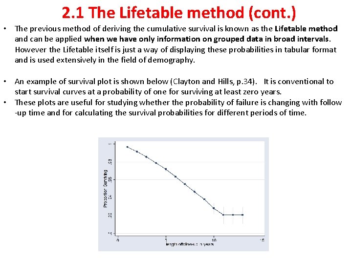
2. 1 The Lifetable method (cont. ) • The previous method of deriving the cumulative survival is known as the Lifetable method and can be applied when we have only information on grouped data in broad intervals. However the Lifetable itself is just a way of displaying these probabilities in tabular format and is used extensively in the field of demography. • An example of survival plot is shown below (Clayton and Hills, p. 34). It is conventional to start survival curves at a probability of one for surviving at least zero years. • These plots are useful for studying whether the probability of failure is changing with follow -up time and for calculating the survival probabilities for different periods of time.

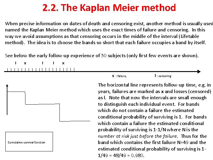
2. 2. The Kaplan Meier method When precise information on dates of death and censoring exist, another method is usually used named the Kaplan Meier method which uses the exact times of failure and censoring. In this way we avoid assumptions as that censoring occurs in the middle of the interval (Lifetable method). The idea is to choose the bands so short that each failure occupies a band by itself. See below the early follow-up experience of 50 subjects (only first few events are shown). l x l l x x : failure, Cumulative survival function l : censoring The horizontal line represents follow-up time, e. g. in years, failures are marked as x and losses (censored) as l. Note that now the intervals are small enough to distinguish each individual event. For bands which do not contain a failure the estimated conditional probability of surviving is 1. For bands which contain a failure the estimated conditional probability of surviving is 1 -1/N where N is the number at risk just before the failure. Thus for the band which contains the first failure N=49 and the estimated conditional probability of surviving is 11/49 = 48/49 = 0. 980.

The cumulative survival probability up to the end of this band i is estimated as S(i) = 1 x 1 x 1. . . x 0. 980 = 0. 980. For the band which contains the second failure N=46 hence the estimated conditional probability of surviving is 1 -1/46 = 45/46. The cumulative probability of surviving up to the end of this band is therefore estimated as: S(i) = 1 x 1 x. . . x 48/49 x 1 x. . x 45/46=0. 980 x 0. 978=0. 958. and so on until there are no more bands which contain failures. The bands containing each failure can be made so short that they refer to the actual time of failure. Then the cumulative survival probability over time takes the value 1 until the first failure then it drops to 0. 980; then it stays at 0. 980 until the time of the second failure where it drops to 0. 958 and so on. The plot of cumulative survival probability vs. time survived takes the stepped shape where steps occur on failure times. If the failure times are measured exactly, the failures will all occur at different times, but if they are measured to the nearest month (for example) then there may be several failures at the same time. In this case the conditional probability of failure is estimated by dividing the number of failures at that failure time by the total number at risk just before the failure time.

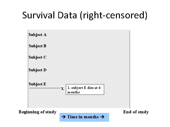
Survival Data (right-censored) Subject A Subject B Subject C Subject D Subject E X 1. subject E dies at 4 months Beginning of study Time in months End of study

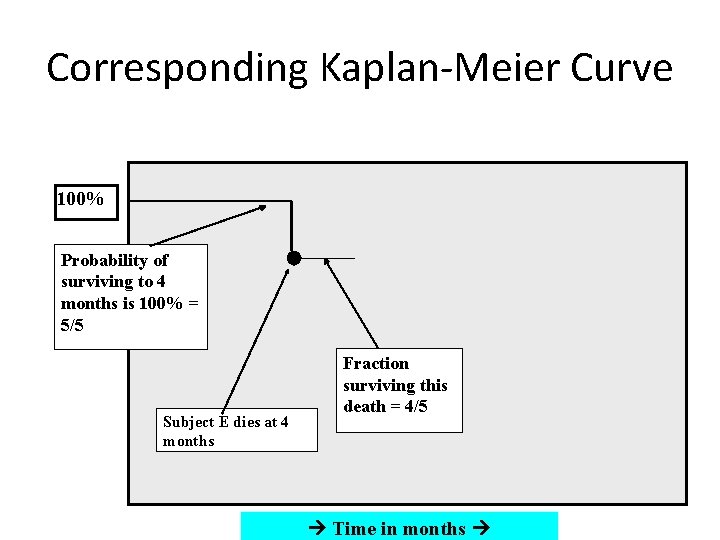
Corresponding Kaplan-Meier Curve 100% Probability of surviving to 4 months is 100% = 5/5 Subject E dies at 4 months Fraction surviving this death = 4/5 Time in months

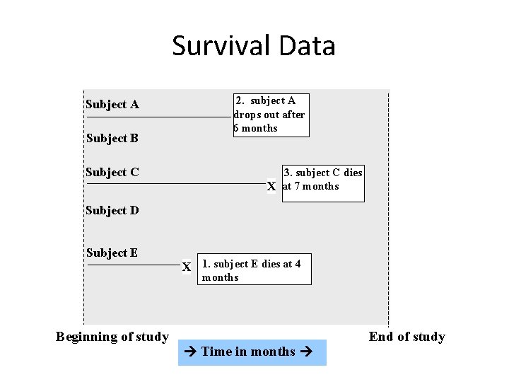
Survival Data Subject A Subject B 2. subject A drops out after 6 months Subject C 3. subject C dies X at 7 months Subject D Subject E X 1. subject E dies at 4 months Beginning of study Time in months End of study

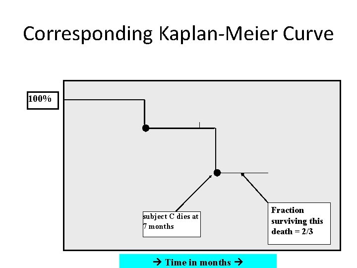
Corresponding Kaplan-Meier Curve 100% subject C dies at 7 months Time in months Fraction surviving this death = 2/3

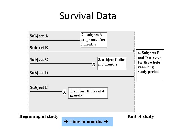
Survival Data Subject A Subject B 2. subject A drops out after 6 months Subject C 3. subject C dies X at 7 months Subject D Subject E 4. Subjects B and D survive for the whole year-long study period X 1. subject E dies at 4 months Beginning of study Time in months End of study

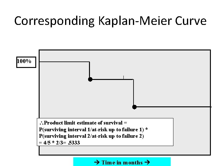
Corresponding Kaplan-Meier Curve 100% Product limit estimate of survival = P(surviving interval 1/at-risk up to failure 1) * P(surviving interval 2/at-risk up to failure 2) = 4/5 * 2/3=. 5333 Time in months

The product limit estimate • The probability of surviving in the entire year, taking into account censoring • = (4/5) (2/3) = 53% • NOTE: 40% (2/5) because the one drop-out survived at least a portion of the year. • AND <60% (3/5) because we don’t know if the one drop-out would have survived until the end of the year.

The Kaplan-Meier Method • In essence, the Kaplan-Meier method is the lifetable method where the interval size is decreased towards zero so that the number of intervals tends to infinity. Each interval has a length just enough for one event or time increment. • Only intervals containing an event contribute to the estimate, so we can ignore all other intervals. • To obtain Kaplan-Meier estimates of survival, the patient survival times are firstly ranked in increasing order. • The times where events (deaths) occur are denoted by ti, where t 1<t 2<t 3<… • The number of deaths occurring at ti is denoted by di.

The Kaplan-Meier Method (cont. ) • If both censoring(s) and death(s) occur at the same time, then the censoring(s) are assumed to occur immediately after the death time. • Censorings do not affect the estimate of S(x), but contribute by decreasing li, the number of person at risk, at the next death time.

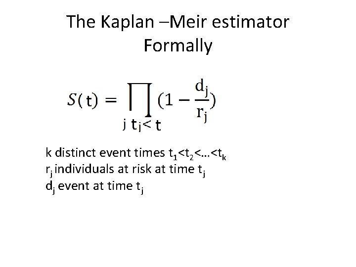
The Kaplan –Meir estimator Formally t t t k distinct event times t 1<t 2<…<tk rj individuals at risk at time tj dj event at time tj

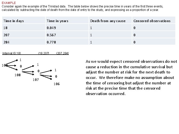
EXAMPLE Consider again the example of the Trinidad data. The table below shows the precise time in years of the first three events, calculated by subtracting the date of death from the date of entry to the study, and expressing as a proportion of a year. Time in days Time in years Death from any cause Censored observations 18 0. 049 1 0 207 0. 567 1 0 284 0. 778 1 0 Interval: (0, 18] 1 109 0 108 (18, 207] (207, 284] 1 0 107 1 0 106 As we would expect censored observations do not cause a reduction in the cumulative survival but adjust the number at risk for the next death to occur. We therefore make no assumption about the time of censoring but adjust the number at risk at the precise time that the censored observation occurred.

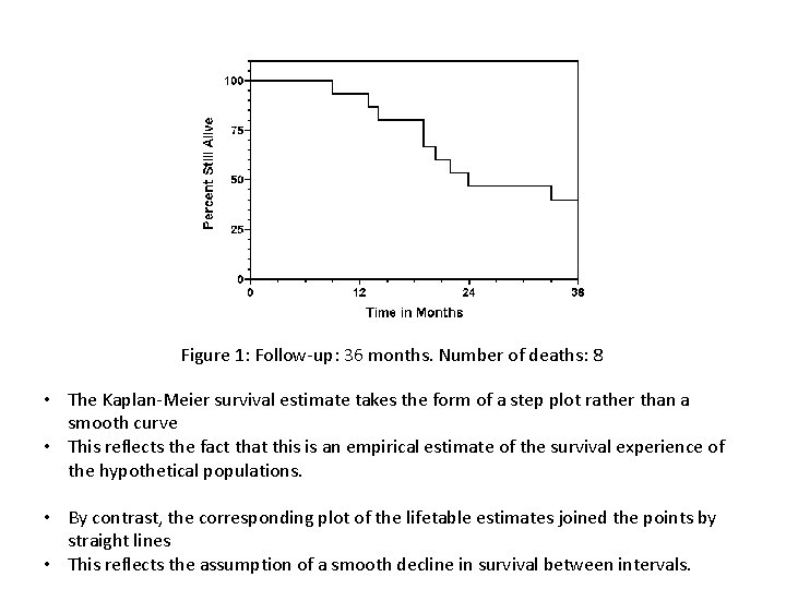
Figure 1: Follow-up: 36 months. Number of deaths: 8 • The Kaplan-Meier survival estimate takes the form of a step plot rather than a smooth curve • This reflects the fact that this is an empirical estimate of the survival experience of the hypothetical populations. • By contrast, the corresponding plot of the lifetable estimates joined the points by straight lines • This reflects the assumption of a smooth decline in survival between intervals.

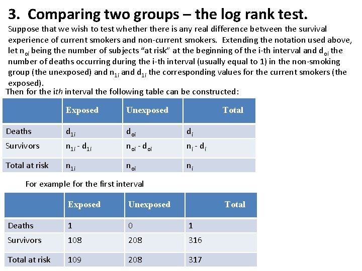
3. Comparing two groups – the log rank test. Suppose that we wish to test whethere is any real difference between the survival experience of current smokers and non-current smokers. Extending the notation used above, let noi being the number of subjects “at risk” at the beginning of the i-th interval and d oi the number of deaths occurring during the i-th interval (usually equal to 1) in the non-smoking group (the unexposed) and n 1 i and d 1 i the corresponding values for the current smokers (the exposed). Then for the ith interval the following table can be constructed: Exposed Unexposed Total Deaths d 1 i doi di Survivors n 1 i - d 1 i noi - doi ni - di Total at risk n 1 i noi ni For example for the first interval Exposed Unexposed Total Deaths 1 0 1 Survivors 108 208 316 Total at risk 109 208 317

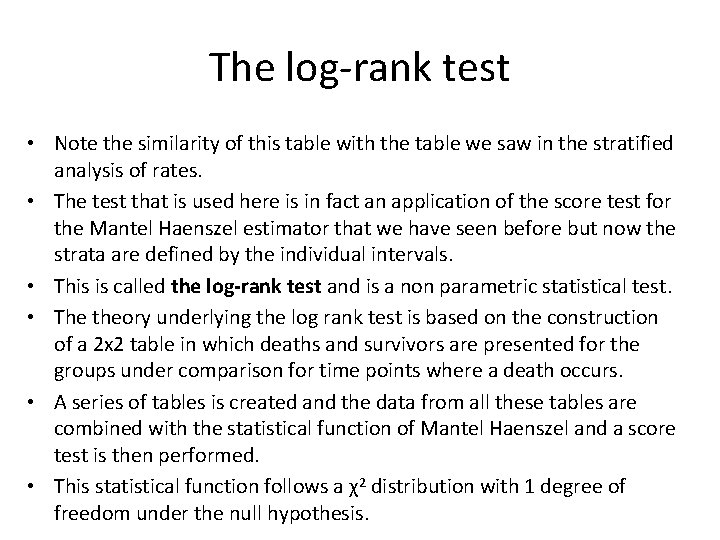
The log-rank test • Note the similarity of this table with the table we saw in the stratified analysis of rates. • The test that is used here is in fact an application of the score test for the Mantel Haenszel estimator that we have seen before but now the strata are defined by the individual intervals. • This is called the log-rank test and is a non parametric statistical test. • The theory underlying the log rank test is based on the construction of a 2 x 2 table in which deaths and survivors are presented for the groups under comparison for time points where a death occurs. • A series of tables is created and the data from all these tables are combined with the statistical function of Mantel Haenszel and a score test is then performed. • This statistical function follows a χ2 distribution with 1 degree of freedom under the null hypothesis.

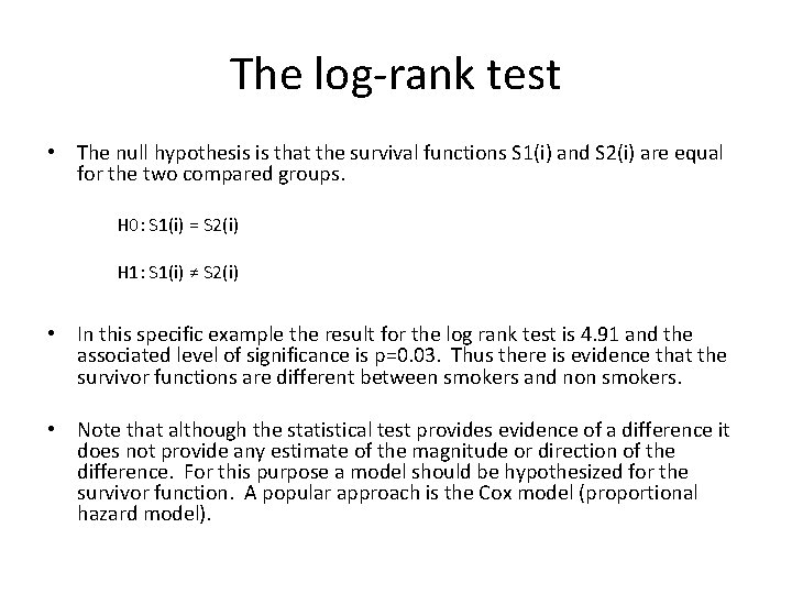
The log-rank test • The null hypothesis is that the survival functions S 1(i) and S 2(i) are equal for the two compared groups. Η 0: S 1(i) = S 2(i) Η 1: S 1(i) ≠ S 2(i) • In this specific example the result for the log rank test is 4. 91 and the associated level of significance is p=0. 03. Thus there is evidence that the survivor functions are different between smokers and non smokers. • Note that although the statistical test provides evidence of a difference it does not provide any estimate of the magnitude or direction of the difference. For this purpose a model should be hypothesized for the survivor function. A popular approach is the Cox model (proportional hazard model).

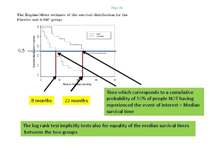
0. 5 8 months 22 months Time which corresponds to a cumulative probability of 50% of people NOT having experienced the event of interest = Median survival time The log rank test implicitly tests also for equality of the median survival times between the two groups

Limitations of Kaplan-Meier • Survival estimates can be unreliable toward the end of a study when there are small numbers of subjects at risk of having an event. • Mainly descriptive • Requires categorical predictors • Can’t accommodate time-dependent variables

Left Censoring • Arises when the event of interest occurred before he/she enters the study; it has already occurred for the individual before observation time. – The survival time is only known to be less than a certain value. – Incomplete nature of the observation occurs in the left tail of the time axis. • Suppose that the event of interest is becoming employed. If a subject is already employed when first interviewed, his outcome is left-censored.

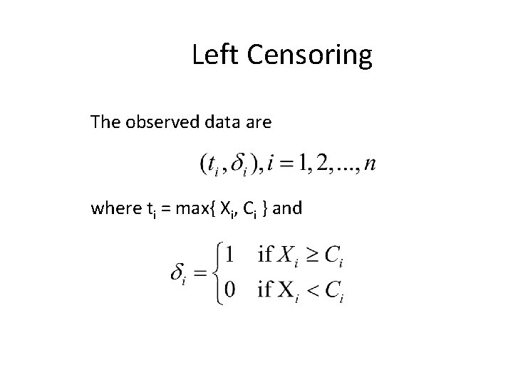
Left Censoring The observed data are where ti = max{ Xi, Ci } and

Left Censoring • In early childhood learning centers interest often focuses upon testing children to determine when a child learns to accomplish certain specified tasks. • The age at which a child learns the task is considered as time to event. • Some children may already perform the task at the study entry. – Such events are considered as left censored.

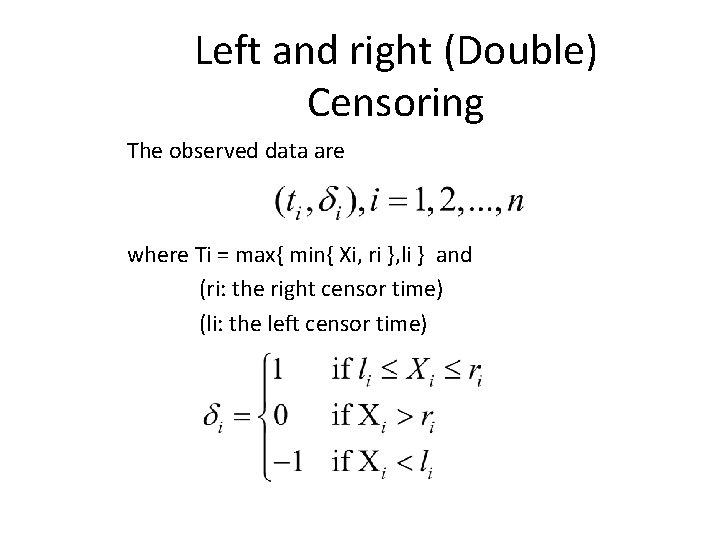
Left and right (Double) Censoring The observed data are where Ti = max{ min{ Xi, ri }, li } and (ri: the right censor time) (li: the left censor time)

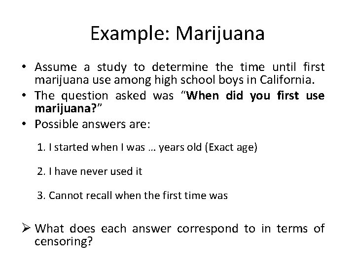
Example: Marijuana • Assume a study to determine the time until first marijuana use among high school boys in California. • The question asked was “When did you first use marijuana? ” • Possible answers are: 1. I started when I was … years old (Exact age) 2. I have never used it 3. Cannot recall when the first time was Ø What does each answer correspond to in terms of censoring?

Interval Censoring • When we only know that failure occurred within an interval, we say data are interval censored. • A generalization of left and right censoring.

Example: The Framingham Heart Study • In the Framingham Study, the ages at which subjects first developed heart disease are usually known exactly. • However the ages of first occurrence of angina pectoris may be known only between two clinical examinations, approximately two years apart.

Truncation • Truncation is a condition which screens out certain subjects so that the investigator will not be aware of their existence. • For truncated data, only subjects who satisfy the condition are observed by the investigator. • The condition is usually associated with a truncation time

Truncation Time • Truncation time for individual i, denoted Yi, is the time of the occurrence of the event truncating individual i.

Left Truncation • Left-truncation occurs when subjects come under observation only if their failure times exceed some time Yi. It is only because they did not fail before Yi that we even knew about their existence. • Only individuals with Xi > Yi are observed. • Left truncated data are rarely seen in medical research; it is often due to the threshold of an apparatus.

Left Truncation • Imagine a study of patients’ survival after surgery • Patients cannot enter the sample until they have had a post-surgical test. • For patients who die before taking the test, survival times will be left-truncated. – This is a “delayed entry” problem, one common type of left-truncation.

Example: Channing House is a retirement center in Palo Alto, CA • For all individuals who lived in the community, ages at death are recorded • Ages at which individuals entered the retirement center are also recorded • Since individuals must survive to a sufficient age to enter the retirement house, individuals who died earlier (i. e. before entering) will never be in the analysis dataset. – They are left truncated

Right Truncation • Arises when only individuals who have experienced the event of interest are included in the sample. • That is, Yi = the end date of study and only individuals with Xi < Yi are observed.

Example: AIDS • Consider an AIDS study. Cases of patients with transfusion-induced AIDS are sampled. • Retrospective determination of the transfusion times were used to estimate the waiting time from infection at transfusion to clinical onset of AIDS • The registry was sampled on 30/6/1986 • Only those developed AIDS before 30/6/1986 were available for observation. – Patients transfused prior to 30/6/1986 who developed AIDS after 30/6/1986 were not observed and were right truncated