Integer Linear Programming ILP Prof KG Satheesh Kumar

Integer Linear Programming (ILP) Prof KG Satheesh Kumar Asian School of Business

Types of ILP Models ILP: A linear program in which some or all variables are restricted to integer values. Types: 1. All-integer LP or a pure ILP 2. Mixed-Integer LP 3. 0 -1 integer LP

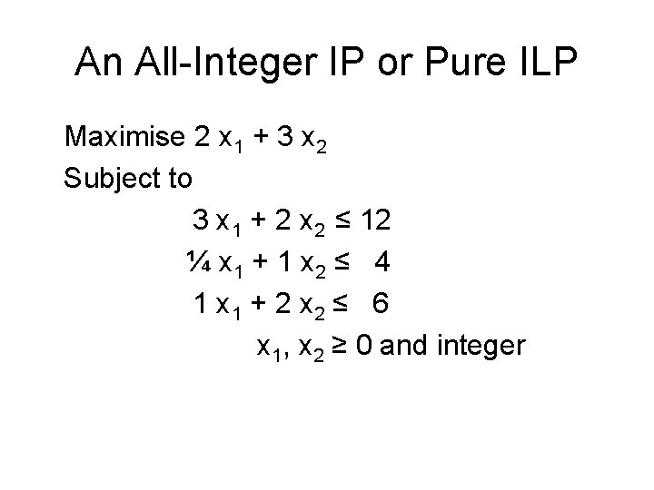
An All-Integer IP or Pure ILP Maximise 2 x 1 + 3 x 2 Subject to 3 x 1 + 2 x 2 ≤ 12 ¼ x 1 + 1 x 2 ≤ 4 1 x 1 + 2 x 2 ≤ 6 x 1, x 2 ≥ 0 and integer

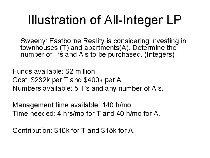
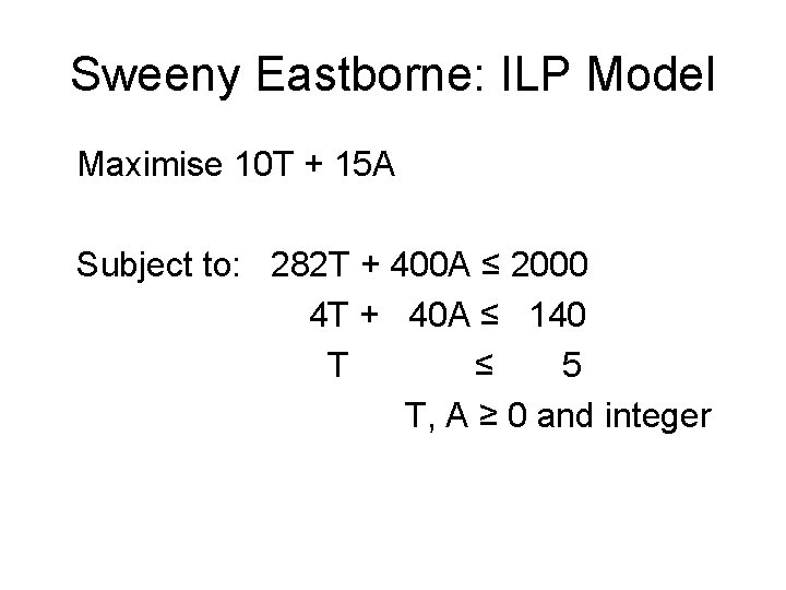
Illustration of All-Integer LP Sweeny: Eastborne Reality is considering investing in townhouses (T) and apartments(A). Determine the number of T’s and A’s to be purchased. (Integers) Funds available: $2 million. Cost: $282 k per T and $400 k per A Numbers available: 5 T’s and any number of A’s. Management time available: 140 h/mo Time needed: 4 hrs/mo for T and 40 h/mo for A. Contribution: $10 k for T and $15 k for A.

Sweeny Eastborne: ILP Model Maximise 10 T + 15 A Subject to: 282 T + 400 A ≤ 2000 4 T + 40 A ≤ 140 T ≤ 5 T, A ≥ 0 and integer

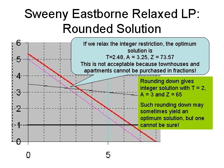
Sweeny Eastborne Relaxed LP: Rounded Solution If we relax the integer restriction, the optimum solution is T=2. 48, A = 3. 25, Z = 73. 57 This is not acceptable because townhouses and apartments cannot be purchased in fractions! Rounding down gives integer solution with T = 2, A = 3 and Z = 65 Such rounding down may sometimes yield an optimum solution, but one cannot be sure!

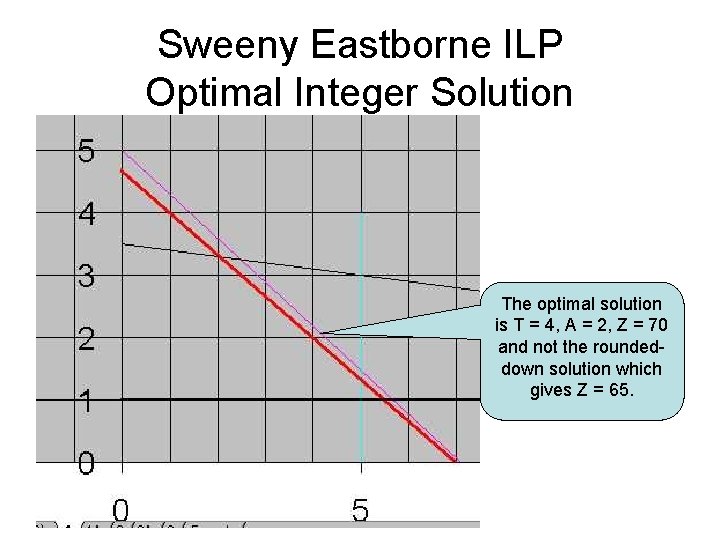
Sweeny Eastborne ILP Optimal Integer Solution The optimal solution is T = 4, A = 2, Z = 70 and not the roundeddown solution which gives Z = 65.

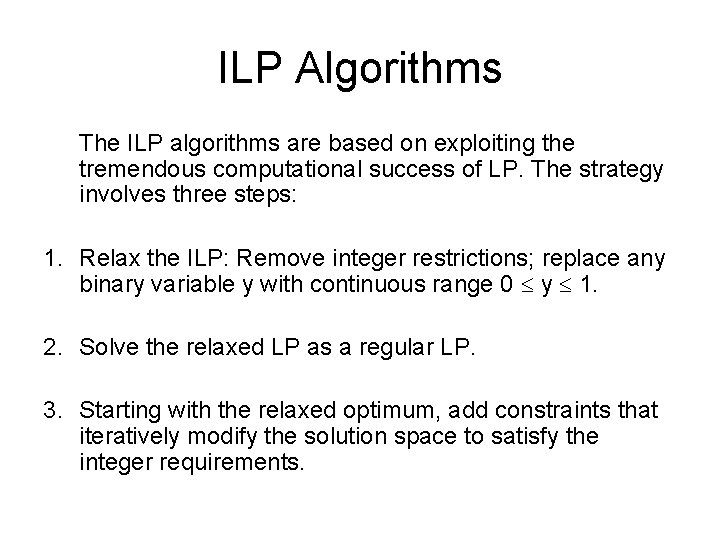
ILP Algorithms The ILP algorithms are based on exploiting the tremendous computational success of LP. The strategy involves three steps: 1. Relax the ILP: Remove integer restrictions; replace any binary variable y with continuous range 0 y 1. 2. Solve the relaxed LP as a regular LP. 3. Starting with the relaxed optimum, add constraints that iteratively modify the solution space to satisfy the integer requirements.

B&B and Cutting Plane Methods The two commonly used methods are: 1. Branch and bound method 2. Cutting Plane Method Neither method is consistently effective; but B&B is far more successful.

Branch-and-Bound (B&B) • Developed in 1960 by A Land G Doig • Relax the integer restrictions in the problem and solve it as a regular LP. Let’s call this LP 0 (to imply node-zero LP) • Test if integer requirements are met. Else branch to get sub-problems LP 1 and LP 2.

Branching • If LP 0 (in general LPi) fails to yield integer solution, branch on any variable that fails to meet this requirement. The process of branching is illustrated below. If LPi yields x 1 = 3. 5 and x 1 is taken as the branching variable, we get two sub-problems, LPi+1 = LPi & (x 1 3) and LPi+2 = LPi & (x 1 4). Note: In mixed integer problems, a continuous variable is never selected for branching.

Bounding / Fathoming • Select LP 1 (in general LPi) and solve. Three conditions arise. – Infeasible solution, declare fathomed (no further investigation of LPi). – Integer solution. If it is superior to the current best solution update the current best. Declare fathomed. – Non-integer solution. If it is inferior to the current best, declare fathomed. Else branch again.

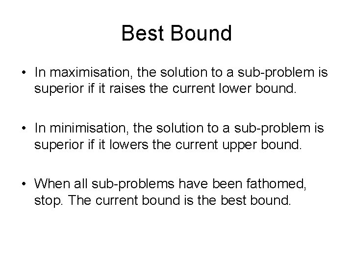
Best Bound • In maximisation, the solution to a sub-problem is superior if it raises the current lower bound. • In minimisation, the solution to a sub-problem is superior if it lowers the current upper bound. • When all sub-problems have been fathomed, stop. The current bound is the best bound.

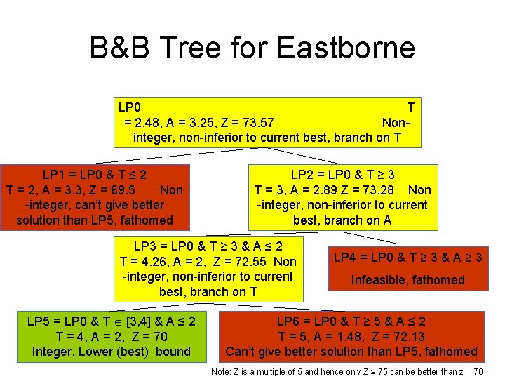
B&B Tree for Eastborne LP 0 T = 2. 48, A = 3. 25, Z = 73. 57 Noninteger, non-inferior to current best, branch on T LP 1 = LP 0 & T ≤ 2 T = 2, A = 3. 3, Z = 69. 5 Non -integer, can’t give better solution than LP 5, fathomed LP 2 = LP 0 & T ≥ 3 T = 3, A = 2. 89 Z = 73. 28 Non -integer, non-inferior to current best, branch on A LP 3 = LP 0 & T ≥ 3 & A ≤ 2 T = 4. 26, A = 2, Z = 72. 55 Non -integer, non-inferior to current best, branch on T LP 5 = LP 0 & T [3, 4] & A ≤ 2 T = 4, A = 2, Z = 70 Integer, Lower (best) bound LP 4 = LP 0 & T ≥ 3 & A ≥ 3 Infeasible, fathomed LP 6 = LP 0 & T ≥ 5 & A ≤ 2 T = 5, A = 1. 48, Z = 72. 13 Can’t give better solution than LP 5, fathomed Note: Z is a multiple of 5 and hence only Z ≥ 75 can be better than z = 70

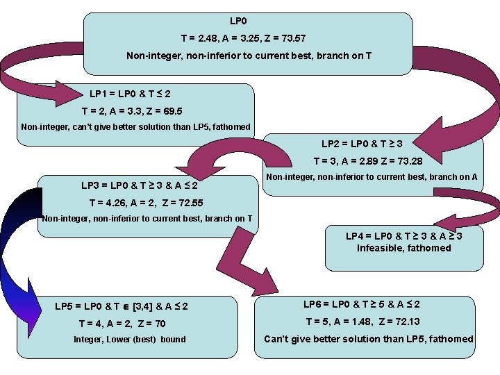
LP 0 T = 2. 48, A = 3. 25, Z = 73. 57 Non-integer, non-inferior to current best, branch on T LP 1 = LP 0 & T ≤ 2 T = 2, A = 3. 3, Z = 69. 5 Non-integer, can’t give better solution than LP 5, fathomed LP 2 = LP 0 & T ≥ 3 T = 3, A = 2. 89 Z = 73. 28 LP 3 = LP 0 & T ≥ 3 & A ≤ 2 Non-integer, non-inferior to current best, branch on A T = 4. 26, A = 2, Z = 72. 55 Non-integer, non-inferior to current best, branch on T LP 4 = LP 0 & T ≥ 3 & A ≥ 3 Infeasible, fathomed LP 5 = LP 0 & T [3, 4] & A ≤ 2 LP 6 = LP 0 & T ≥ 5 & A ≤ 2 T = 4, A = 2, Z = 70 T = 5, A = 1. 48, Z = 72. 13 Integer, Lower (best) bound Can’t give better solution than LP 5, fathomed

See more illustrations of Branch-and-Bound algorithm in the Excel sheet

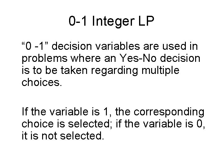
0 -1 Integer LP “ 0 -1” decision variables are used in problems where an Yes-No decision is to be taken regarding multiple choices. If the variable is 1, the corresponding choice is selected; if the variable is 0, it is not selected.

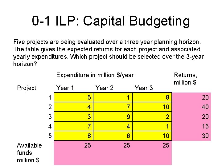
0 -1 ILP: Capital Budgeting Five projects are being evaluated over a three year planning horizon. The table gives the expected returns for each project and associated yearly expenditures. Which project should be selected over the 3 -year horizon? Expenditure in million $/year Project Available funds, million $ Year 1 Year 2 Returns, million $ Year 3 1 5 1 8 20 2 4 7 10 40 3 3 9 2 20 4 7 4 1 15 5 8 6 10 30 25 25 25

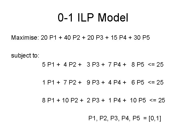
0 -1 ILP Model Maximise: 20 P 1 + 40 P 2 + 20 P 3 + 15 P 4 + 30 P 5 subject to: 5 P 1 + 4 P 2 + 3 P 3 + 7 P 4 + 8 P 5 <= 25 1 P 1 + 7 P 2 + 9 P 3 + 4 P 4 + 6 P 5 <= 25 8 P 1 + 10 P 2 + 2 P 3 + 1 P 4 + 10 P 5 <= 25 P 1, P 2, P 3, P 4, P 5 = [0, 1]

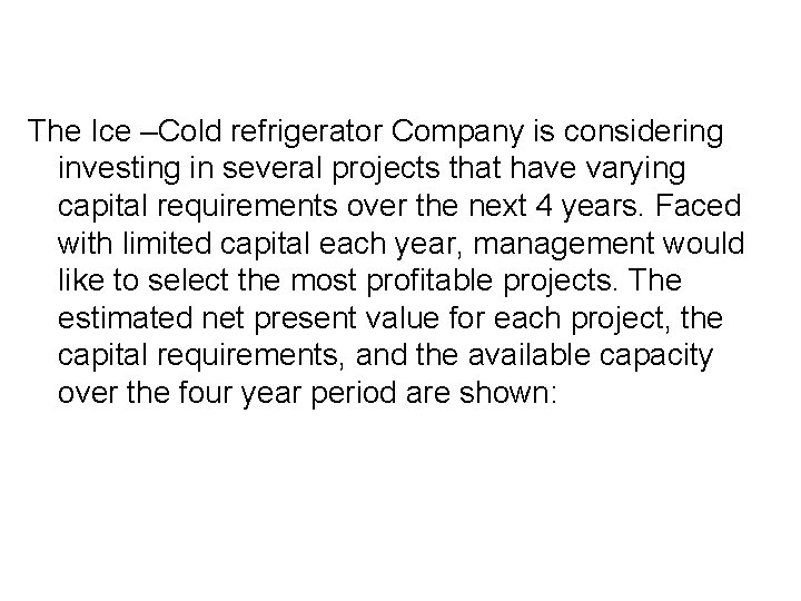
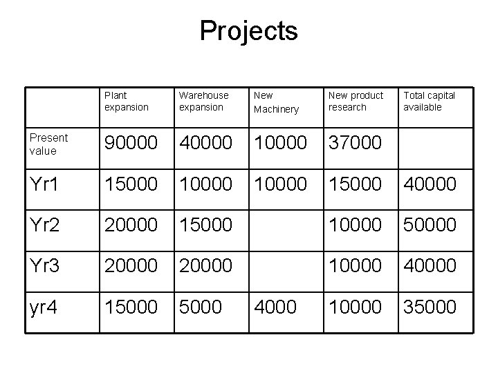
The Ice –Cold refrigerator Company is considering investing in several projects that have varying capital requirements over the next 4 years. Faced with limited capital each year, management would like to select the most profitable projects. The estimated net present value for each project, the capital requirements, and the available capacity over the four year period are shown:

Projects Plant expansion Warehouse expansion New Machinery New product research Present value 90000 40000 10000 37000 Yr 1 15000 10000 15000 40000 Yr 2 20000 15000 10000 50000 Yr 3 20000 10000 40000 yr 4 15000 10000 35000 4000 Total capital available

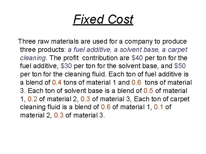
Fixed Cost Three raw materials are used for a company to produce three products: a fuel additive, a solvent base, a carpet cleaning. The profit contribution are $40 per ton for the fuel additive, $30 per ton for the solvent base, and $50 per ton for the cleaning fluid. Each ton of fuel additive is a blend of 0. 4 tons of material 1 and 0. 6 tons of material 3. Each ton of solvent base is a blend of 0. 5 of material 1, 0. 2 of material 2, 0. 3 of material 3, Each ton of carpet cleaning fluid is a blend of 0. 6 of material 1, 0. 1 of material 2, 0. 3 of material 3.

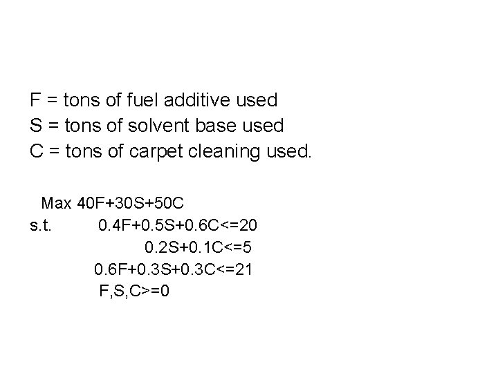
F = tons of fuel additive used S = tons of solvent base used C = tons of carpet cleaning used. Max 40 F+30 S+50 C s. t. 0. 4 F+0. 5 S+0. 6 C<=20 0. 2 S+0. 1 C<=5 0. 6 F+0. 3 S+0. 3 C<=21 F, S, C>=0

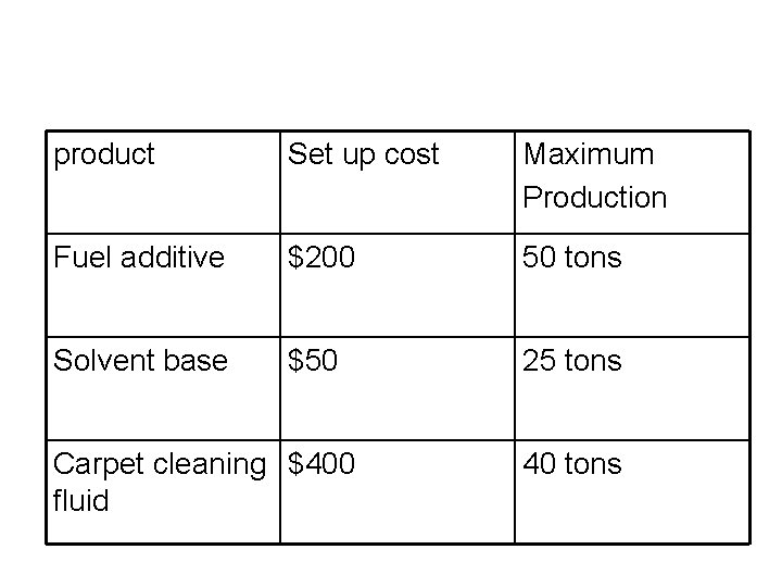
product Set up cost Maximum Production Fuel additive $200 50 tons Solvent base $50 25 tons Carpet cleaning $400 fluid 40 tons

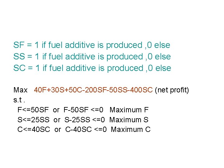
SF = 1 if fuel additive is produced , 0 else SS = 1 if fuel additive is produced , 0 else SC = 1 if fuel additive is produced , 0 else Max 40 F+30 S+50 C-200 SF-50 SS-400 SC (net profit) s. t. F<=50 SF or F-50 SF <=0 Maximum F S<=25 SS or S-25 SS <=0 Maximum S C<=40 SC or C-40 SC <=0 Maximum C

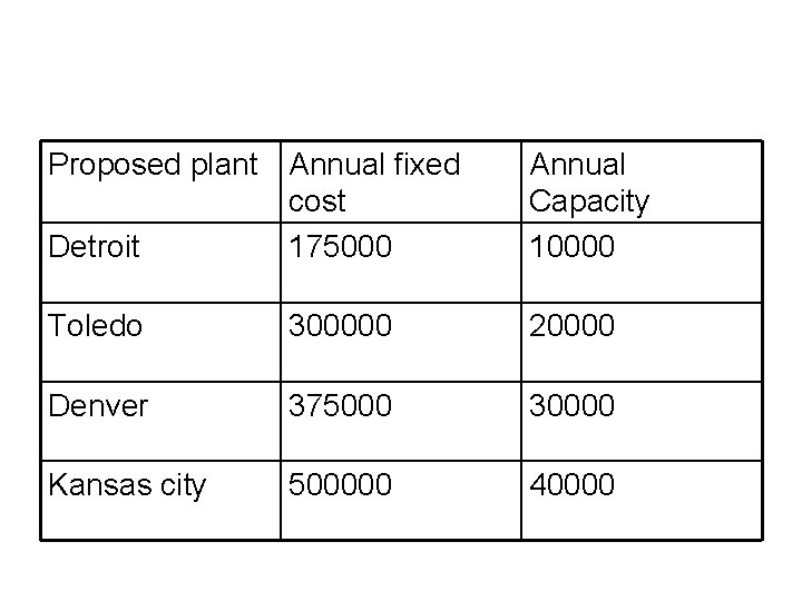
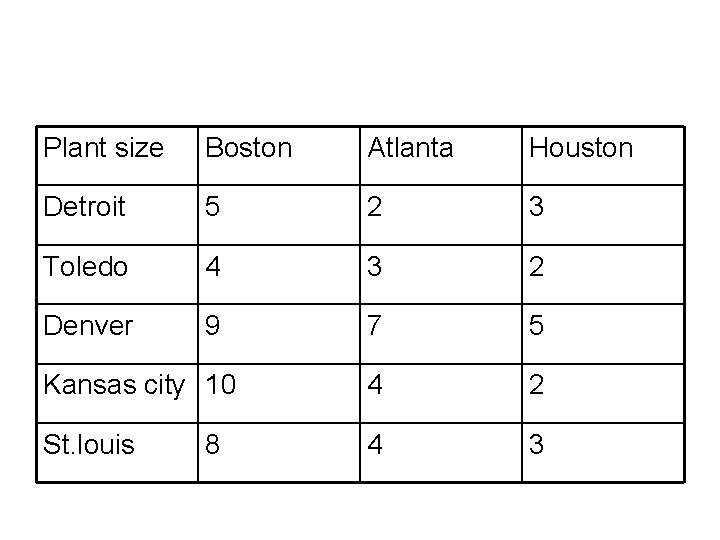
Distribution Systems Design The Martin-Beck Company operates a plant in St. Louis with an annual capacity of 30, 000 units. Product is shipped to regional centers located in Boston, Atlanta, Houston. Bcos of an anticipated increase in demand, Martin-Beck plans to increase the capacity by constructing a new plant in one or more of the following cities : Detroit, Toledo, Denver or Kansas City. The estimated annual fixed cost and the annual capacity for the 4 proposed plants is as follows:

Proposed plant Annual fixed cost Detroit 175000 Annual Capacity 10000 Toledo 300000 20000 Denver 375000 30000 Kansas city 500000 40000

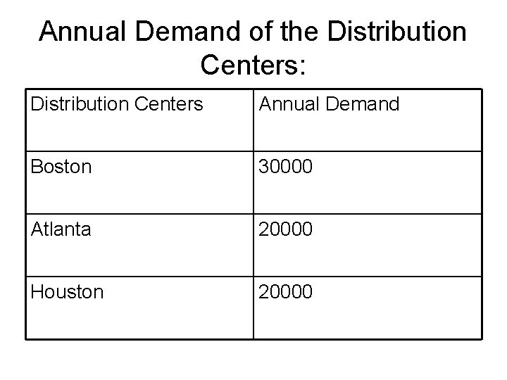
Annual Demand of the Distribution Centers: Distribution Centers Annual Demand Boston 30000 Atlanta 20000 Houston 20000

Plant size Boston Atlanta Houston Detroit 5 2 3 Toledo 4 3 2 Denver 9 7 5 Kansas city 10 4 2 St. louis 4 3 8

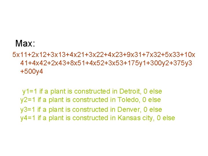
Max: 5 x 11+2 x 12+3 x 13+4 x 21+3 x 22+4 x 23+9 x 31+7 x 32+5 x 33+10 x 41+4 x 42+2 x 43+8 x 51+4 x 52+3 x 53+175 y 1+300 y 2+375 y 3 +500 y 4 y 1=1 if a plant is constructed in Detroit, 0 else y 2=1 if a plant is constructed in Toledo, 0 else y 3=1 if a plant is constructed in Denver, 0 else y 4=1 if a plant is constructed in Kansas city, 0 else

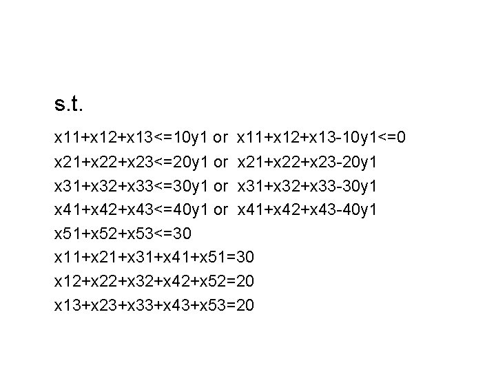
s. t. x 11+x 12+x 13<=10 y 1 or x 11+x 12+x 13 -10 y 1<=0 x 21+x 22+x 23<=20 y 1 or x 21+x 22+x 23 -20 y 1 x 31+x 32+x 33<=30 y 1 or x 31+x 32+x 33 -30 y 1 x 41+x 42+x 43<=40 y 1 or x 41+x 42+x 43 -40 y 1 x 51+x 52+x 53<=30 x 11+x 21+x 31+x 41+x 51=30 x 12+x 22+x 32+x 42+x 52=20 x 13+x 23+x 33+x 43+x 53=20

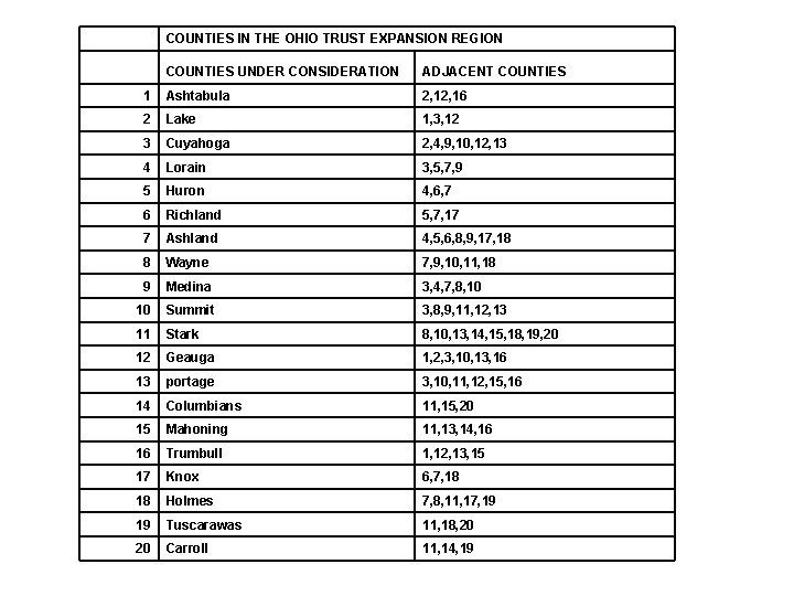
Branch Location • The long-range planning department for the Ohio Trust Company is considering expanding its operation into a 20 -county region in NE Ohio. Currently, Ohio Trust does not have a principal place of business in any of the 20 counties. According to the banking laws in Ohio, if a bank establishes a principal place of business (PPB) in any county, branch banks can be estd in that county and in any adjacent county. However, to establish a new PPB, Ohio Trust must either obtain approval for a new bank from the state’s superintendent of banks or purchase an existing bank.

COUNTIES IN THE OHIO TRUST EXPANSION REGION COUNTIES UNDER CONSIDERATION ADJACENT COUNTIES 1 Ashtabula 2, 16 2 Lake 1, 3, 12 3 Cuyahoga 2, 4, 9, 10, 12, 13 4 Lorain 3, 5, 7, 9 5 Huron 4, 6, 7 6 Richland 5, 7, 17 7 Ashland 4, 5, 6, 8, 9, 17, 18 8 Wayne 7, 9, 10, 11, 18 9 Medina 3, 4, 7, 8, 10 10 Summit 3, 8, 9, 11, 12, 13 11 Stark 8, 10, 13, 14, 15, 18, 19, 20 12 Geauga 1, 2, 3, 10, 13, 16 13 portage 3, 10, 11, 12, 15, 16 14 Columbians 11, 15, 20 15 Mahoning 11, 13, 14, 16 16 Trumbull 1, 12, 13, 15 17 Knox 6, 7, 18 18 Holmes 7, 8, 11, 17, 19 19 Tuscarawas 11, 18, 20 20 Carroll 11, 14, 19

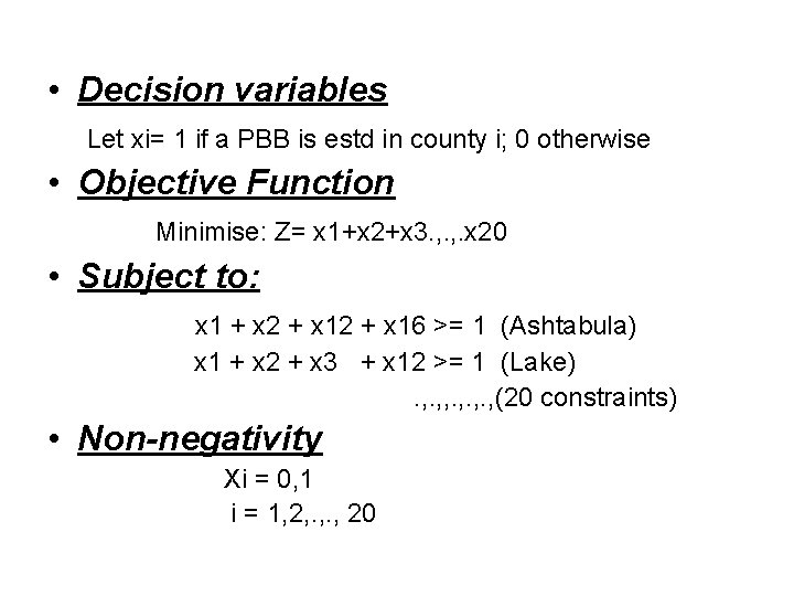
• Decision variables Let xi= 1 if a PBB is estd in county i; 0 otherwise • Objective Function Minimise: Z= x 1+x 2+x 3. , . x 20 • Subject to: x 1 + x 2 + x 16 >= 1 (Ashtabula) x 1 + x 2 + x 3 + x 12 >= 1 (Lake). , , . , . , (20 constraints) • Non-negativity Xi = 0, 1 i = 1, 2, . , 20

See more illustrations of 0 -1 ILP and solution using Excel Solver

Reference • Hamdy A Taha, “Operations Research: An Introduction”; Pearson • Anderson, Sweeny and Williams, “An Introduction to Management Science”; Thomson Thank you for listening