Chapter 15 Integer Optimization Integer Optimization An integer

Chapter 15 Integer Optimization

Integer Optimization An integer linear optimization model (integer program) has some or all variables restricted to being whole numbers. A mixed-integer linear optimization model has only a subset of variables restricted to being integer while others are continuous. A special type of integer problem is one in which variables can be only 0 or 1; these are used to model logical yes-or-no decisions.

Solving Models with General Integer Variables Decision variables that we force to be integers are called general integer variables. Algorithms for integer optimization models first solve the LP relaxation (no integer restrictions imposed) and gradually enforce integer restrictions using systematic searches. Solver has a default integer tolerance of 0. 05 so it will stop if it finds an integer solution within 5% of the optimal solution. ◦ To find the guaranteed optimal integer solution, Integer Tolerance must be set to 0. Click the Options button in the Solver Parameters dialog and ensure that the value of Integer Optimality (%) is 0.

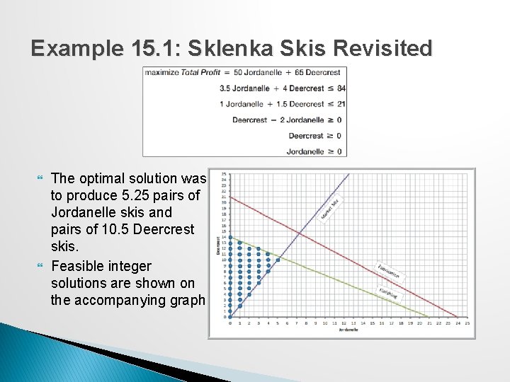
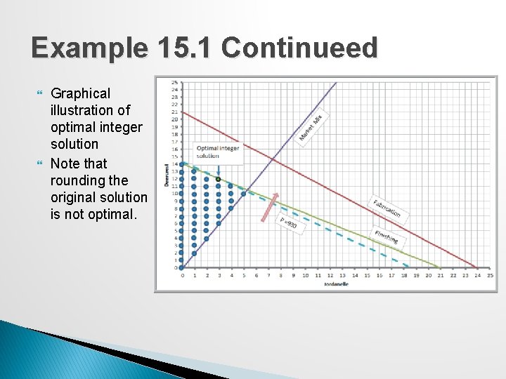
Example 15. 1: Sklenka Skis Revisited The optimal solution was to produce 5. 25 pairs of Jordanelle skis and pairs of 10. 5 Deercrest skis. Feasible integer solutions are shown on the accompanying graph.

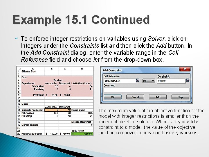
Example 15. 1 Continued To enforce integer restrictions on variables using Solver, click on Integers under the Constraints list and then click the Add button. In the Add Constraint dialog, enter the variable range in the Cell Reference field and choose int from the drop-down box. The maximum value of the objective function for the model with integer restrictions is smaller than the linear optimization solution. Whenever you add a constraint to a model, the value of the objective function can never improve and usually worsens.

Example 15. 1 Continueed Graphical illustration of optimal integer solution Note that rounding the original solution is not optimal.

Sensitivity Analysis for Integer Optimization Because integer models are discontinuous by their very nature, sensitivity information cannot be generated in the same manner as for linear models; therefore, no Sensitivity report is provided by Solver— only the Answer report is available. To investigate changes in model parameters, it is necessary to re-solve the model.

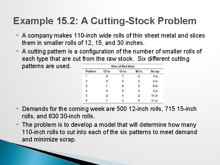
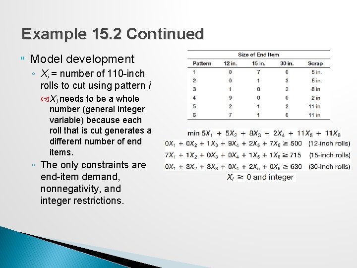
Example 15. 2: A Cutting-Stock Problem A company makes 110 -inch wide rolls of thin sheet metal and slices them in smaller rolls of 12, 15, and 30 inches. A cutting pattern is a configuration of the number of smaller rolls of each type that are cut from the raw stock. Six different cutting patterns are used. Demands for the coming week are 500 12 -inch rolls, 715 15 -inch rolls, and 630 30 -inch rolls. The problem is to develop a model that will determine how many 110 -inch rolls to cut into each of the six patterns to meet demand minimize scrap.

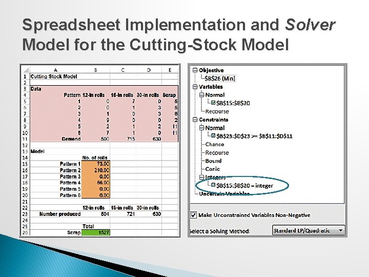
Example 15. 2 Continued Model development ◦ Xi = number of 110 -inch rolls to cut using pattern i Xi needs to be a whole number (general integer variable) because each roll that is cut generates a different number of end items. ◦ The only constraints are end-item demand, nonnegativity, and integer restrictions.

Spreadsheet Implementation and Solver Model for the Cutting-Stock Model

Workforce-Scheduling Models Workforce scheduling is a practical, yet highly complex, problem in many businesses such as food service, hospitals, and airlines. Typically a huge number of possible schedules exist and customer demand varies by day of week and time of day, further complicating the problem of assigning workers to time slots.

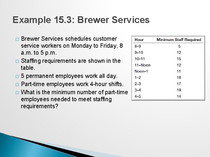
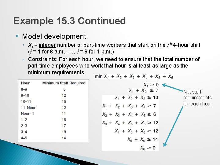
Example 15. 3: Brewer Services � � � Brewer Services schedules customer service workers on Monday to Friday, 8 a. m. to 5 p. m. Staffing requirements are shown in the table. 5 permanent employees work all day. Part-time employees work 4 -hour shifts. What is the minimum number of part-time employees needed to meet staffing requirements?

Example 15. 3 Continued Model development ◦ Xi = integer number of part-time workers that start on the ith 4 -hour shift (i = 1 for 8 a. m. , …, i = 6 for 1 p. m. ) ◦ Constraints: For each hour, we need to ensure that the total number of part-time employees who work that hour is at least as large as the minimum requirements. Net staff requirements for each hour

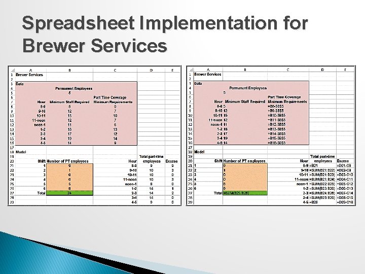
Spreadsheet Implementation for Brewer Services

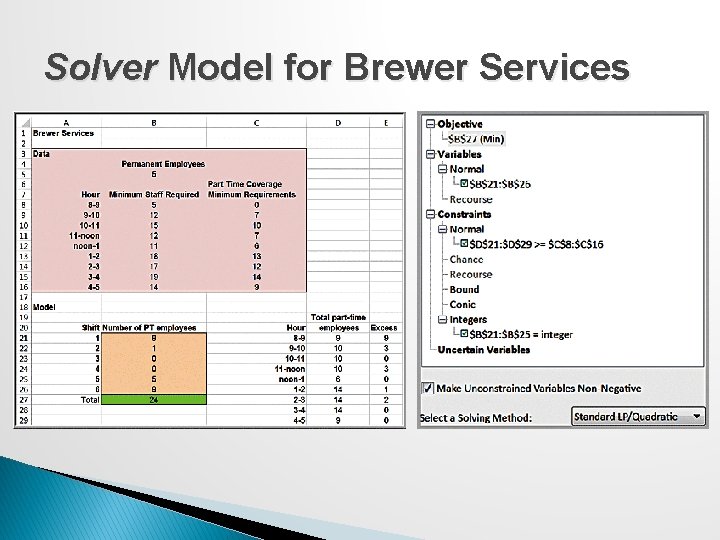
Solver Model for Brewer Services

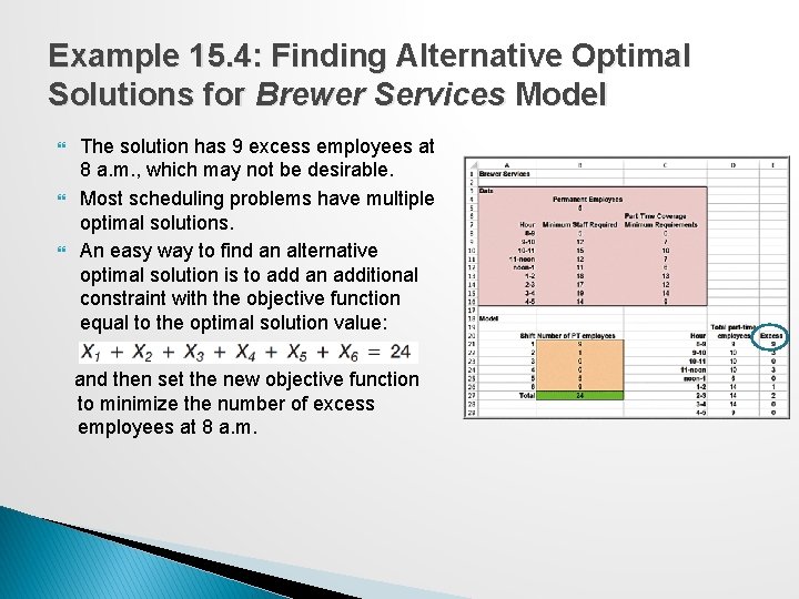
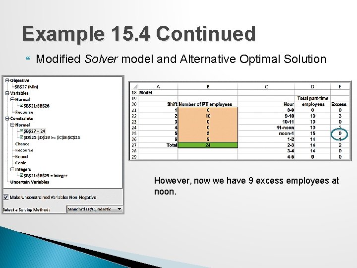
Example 15. 4: Finding Alternative Optimal Solutions for Brewer Services Model The solution has 9 excess employees at 8 a. m. , which may not be desirable. Most scheduling problems have multiple optimal solutions. An easy way to find an alternative optimal solution is to add an additional constraint with the objective function equal to the optimal solution value: and then set the new objective function to minimize the number of excess employees at 8 a. m.

Example 15. 4 Continued Modified Solver model and Alternative Optimal Solution However, now we have 9 excess employees at noon.

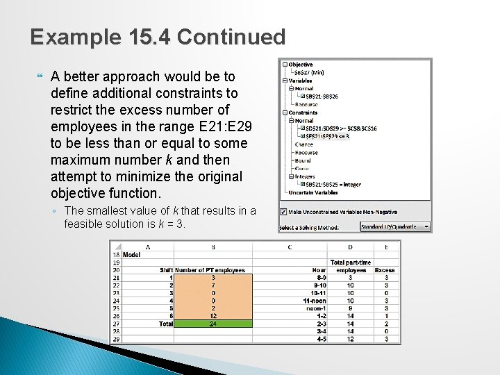
Example 15. 4 Continued A better approach would be to define additional constraints to restrict the excess number of employees in the range E 21: E 29 to be less than or equal to some maximum number k and then attempt to minimize the original objective function. ◦ The smallest value of k that results in a feasible solution is k = 3.

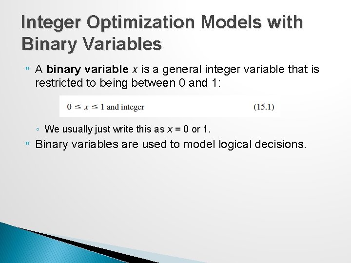
Integer Optimization Models with Binary Variables A binary variable x is a general integer variable that is restricted to being between 0 and 1: ◦ We usually just write this as x = 0 or 1. Binary variables are used to model logical decisions.

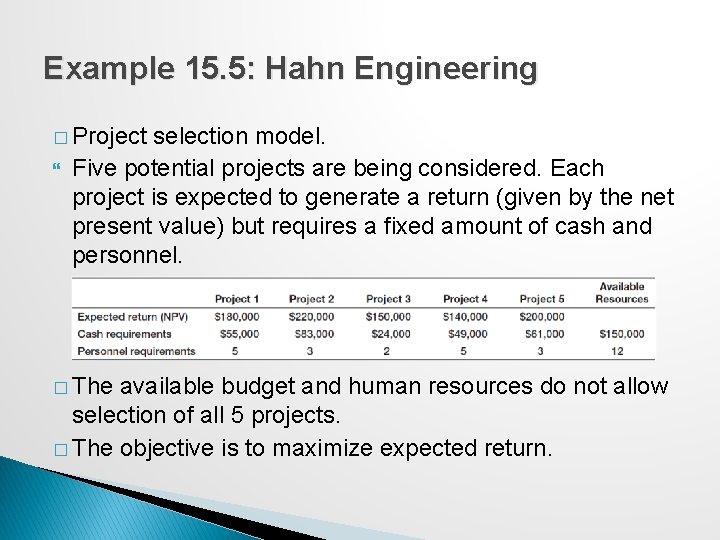
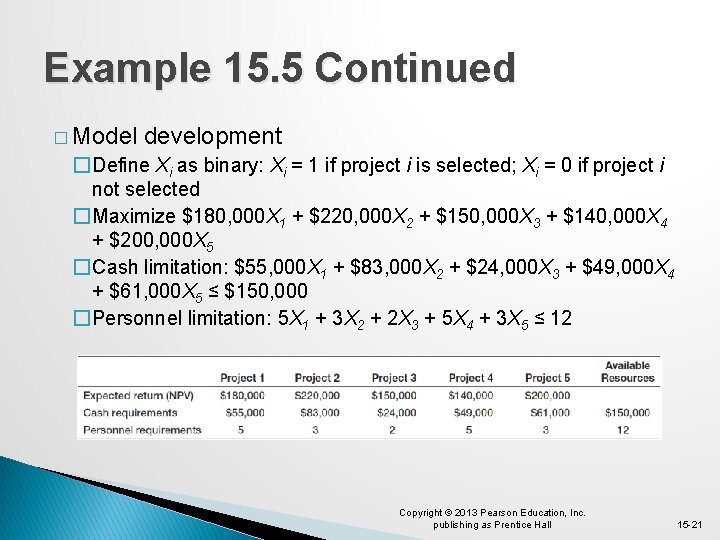
Example 15. 5: Hahn Engineering � Project selection model. Five potential projects are being considered. Each project is expected to generate a return (given by the net present value) but requires a fixed amount of cash and personnel. � The available budget and human resources do not allow selection of all 5 projects. � The objective is to maximize expected return.

Example 15. 5 Continued � Model development �Define Xi as binary: Xi = 1 if project i is selected; Xi = 0 if project i not selected �Maximize $180, 000 X 1 + $220, 000 X 2 + $150, 000 X 3 + $140, 000 X 4 + $200, 000 X 5 �Cash limitation: $55, 000 X 1 + $83, 000 X 2 + $24, 000 X 3 + $49, 000 X 4 + $61, 000 X 5 ≤ $150, 000 �Personnel limitation: 5 X 1 + 3 X 2 + 2 X 3 + 5 X 4 + 3 X 5 ≤ 12 Copyright © 2013 Pearson Education, Inc. publishing as Prentice Hall 15 -21

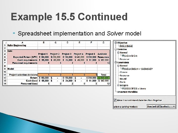
Example 15. 5 Continued Spreadsheet implementation and Solver model

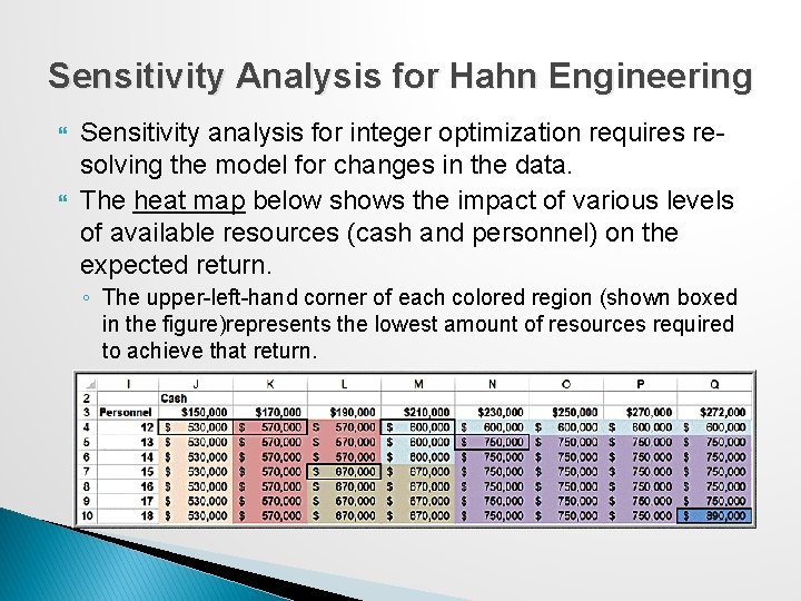
Sensitivity Analysis for Hahn Engineering Sensitivity analysis for integer optimization requires resolving the model for changes in the data. The heat map below shows the impact of various levels of available resources (cash and personnel) on the expected return. ◦ The upper-left-hand corner of each colored region (shown boxed in the figure)represents the lowest amount of resources required to achieve that return.

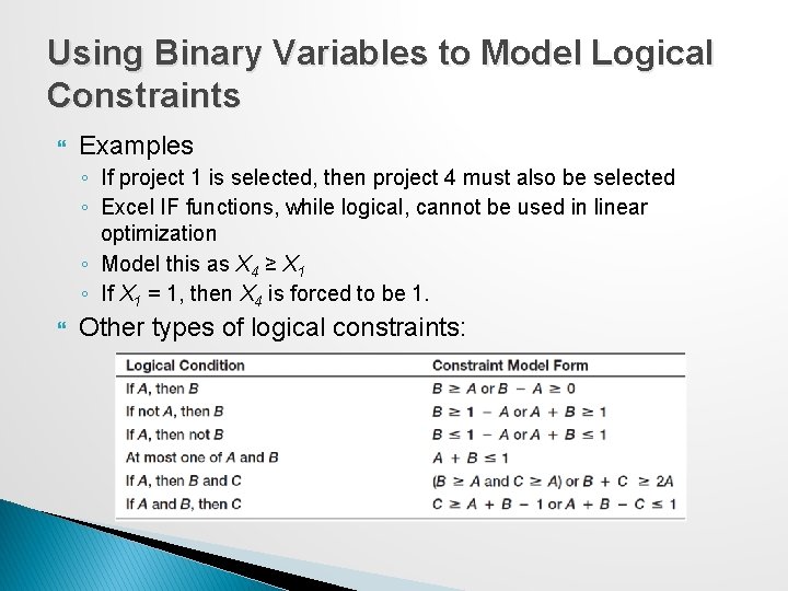
Using Binary Variables to Model Logical Constraints Examples ◦ If project 1 is selected, then project 4 must also be selected ◦ Excel IF functions, while logical, cannot be used in linear optimization ◦ Model this as X 4 ≥ X 1 ◦ If X 1 = 1, then X 4 is forced to be 1. Other types of logical constraints:

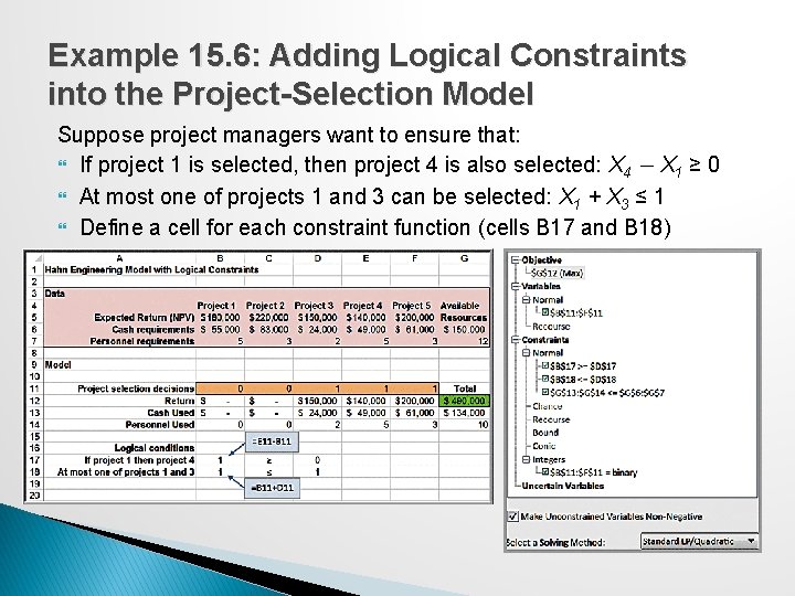
Example 15. 6: Adding Logical Constraints into the Project-Selection Model Suppose project managers want to ensure that: If project 1 is selected, then project 4 is also selected: X 4 − X 1 ≥ 0 At most one of projects 1 and 3 can be selected: X 1 + X 3 ≤ 1 Define a cell for each constraint function (cells B 17 and B 18)

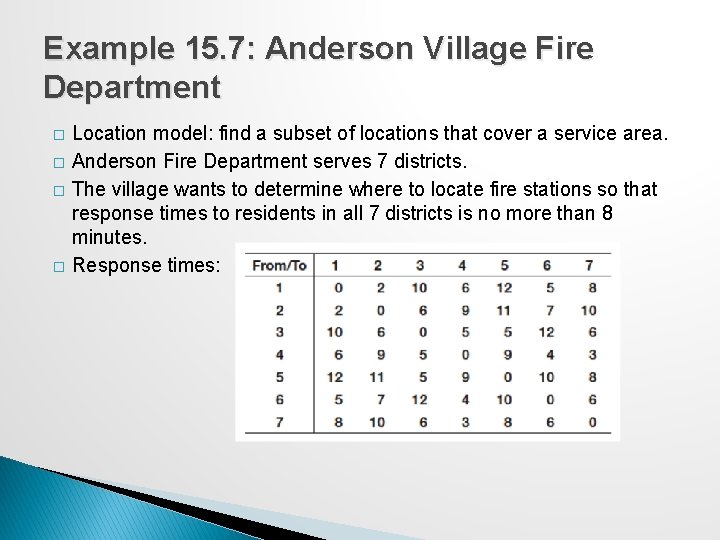
Example 15. 7: Anderson Village Fire Department � � Location model: find a subset of locations that cover a service area. Anderson Fire Department serves 7 districts. The village wants to determine where to locate fire stations so that response times to residents in all 7 districts is no more than 8 minutes. Response times:

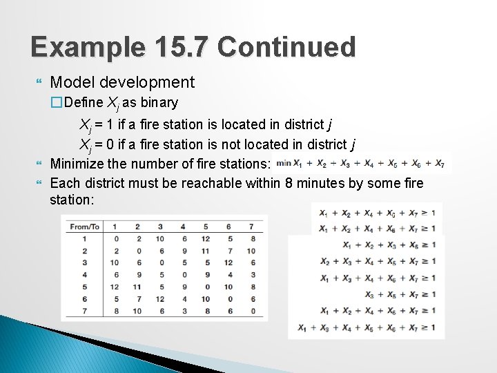
Example 15. 7 Continued Model development �Define Xj as binary Xj = 1 if a fire station is located in district j Xj = 0 if a fire station is not located in district j Minimize the number of fire stations: Each district must be reachable within 8 minutes by some fire station:

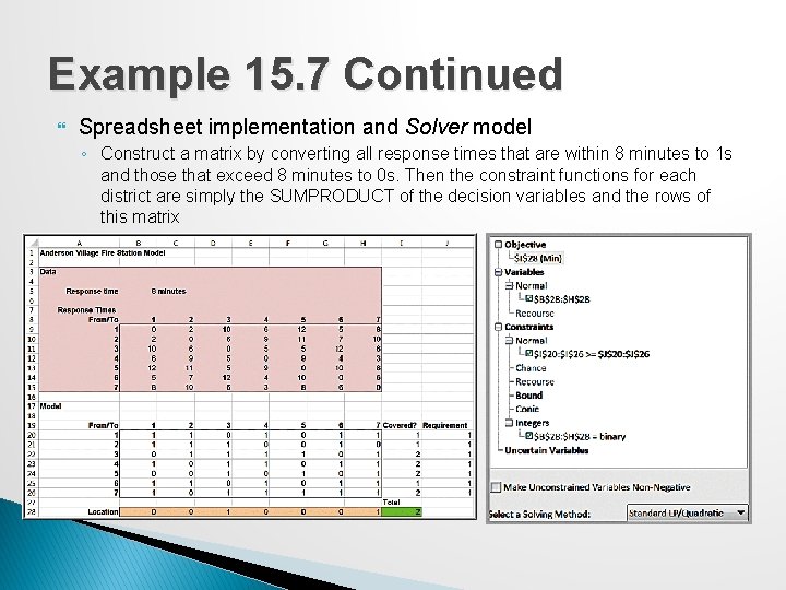
Example 15. 7 Continued Spreadsheet implementation and Solver model ◦ Construct a matrix by converting all response times that are within 8 minutes to 1 s and those that exceed 8 minutes to 0 s. Then the constraint functions for each district are simply the SUMPRODUCT of the decision variables and the rows of this matrix

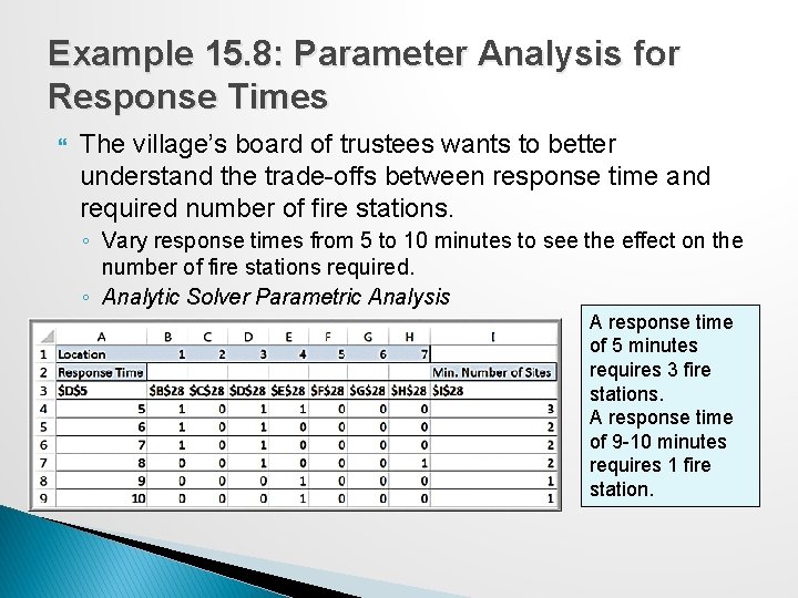
Example 15. 8: Parameter Analysis for Response Times The village’s board of trustees wants to better understand the trade-offs between response time and required number of fire stations. ◦ Vary response times from 5 to 10 minutes to see the effect on the number of fire stations required. ◦ Analytic Solver Parametric Analysis A response time of 5 minutes requires 3 fire stations. A response time of 9 -10 minutes requires 1 fire station.

A Customer-Assignment Model for Supply Chain Optimization A company has numerous potential locations for distribution centers to ship products to customers. A single-sourcing policy specifies that each customer can only be supplied from one distribution center. The problem is to determine which customers to assign to each distribution center.

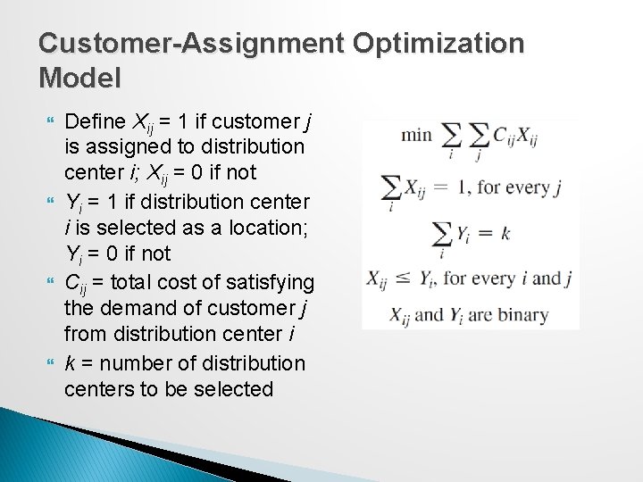
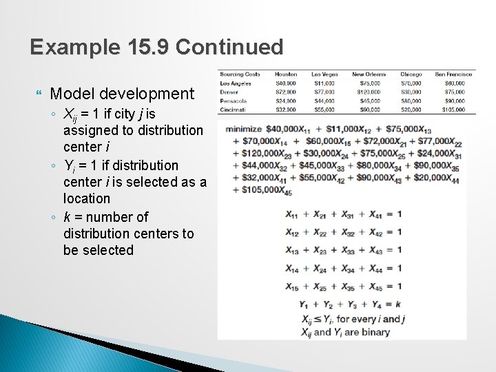
Customer-Assignment Optimization Model Define Xij = 1 if customer j is assigned to distribution center i; Xij = 0 if not Yi = 1 if distribution center i is selected as a location; Yi = 0 if not Cij = total cost of satisfying the demand of customer j from distribution center i k = number of distribution centers to be selected

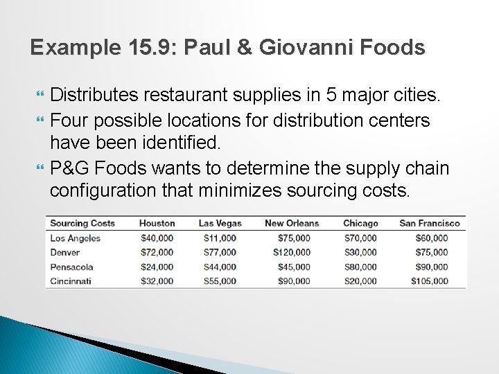
Example 15. 9: Paul & Giovanni Foods Distributes restaurant supplies in 5 major cities. Four possible locations for distribution centers have been identified. P&G Foods wants to determine the supply chain configuration that minimizes sourcing costs.

Example 15. 9 Continued Model development ◦ Xij = 1 if city j is assigned to distribution center i ◦ Yi = 1 if distribution center i is selected as a location ◦ k = number of distribution centers to be selected

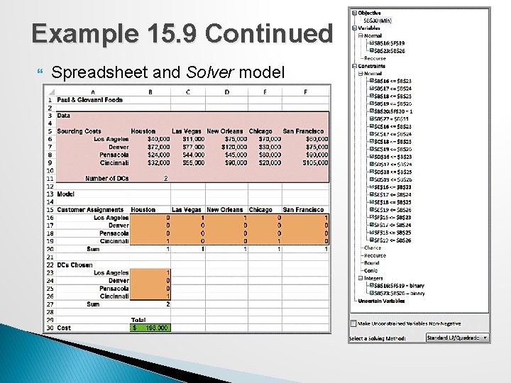
Example 15. 9 Continued Spreadsheet and Solver model

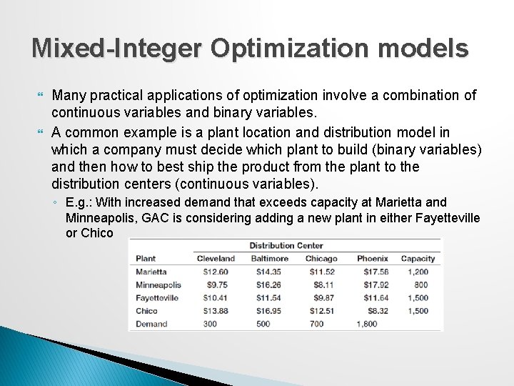
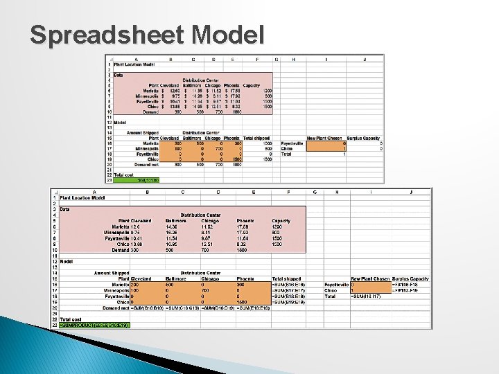
Mixed-Integer Optimization models Many practical applications of optimization involve a combination of continuous variables and binary variables. A common example is a plant location and distribution model in which a company must decide which plant to build (binary variables) and then how to best ship the product from the plant to the distribution centers (continuous variables). ◦ E. g. : With increased demand that exceeds capacity at Marietta and Minneapolis, GAC is considering adding a new plant in either Fayetteville or Chico

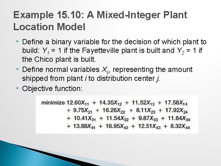
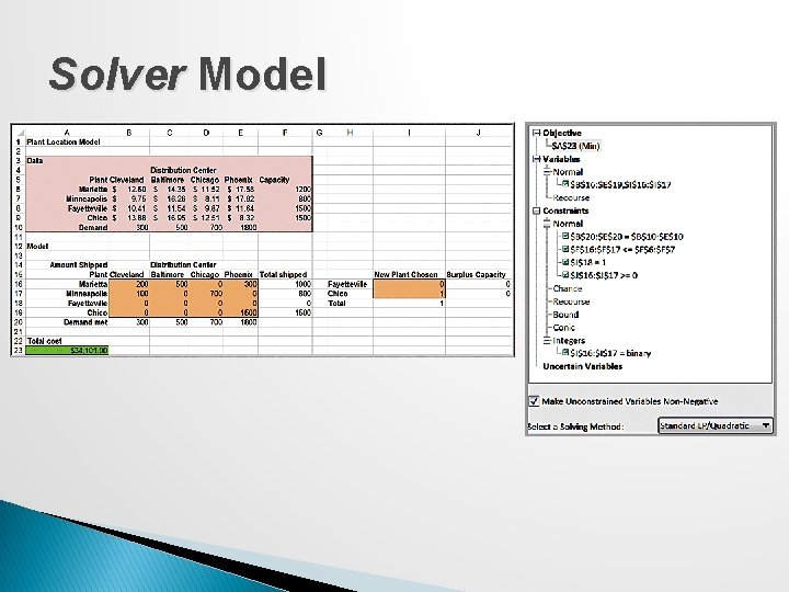
Example 15. 10: A Mixed-Integer Plant Location Model Define a binary variable for the decision of which plant to build: Y 1 = 1 if the Fayetteville plant is built and Y 2 = 1 if the Chico plant is built. Define normal variables Xij, representing the amount shipped from plant i to distribution center j. Objective function:

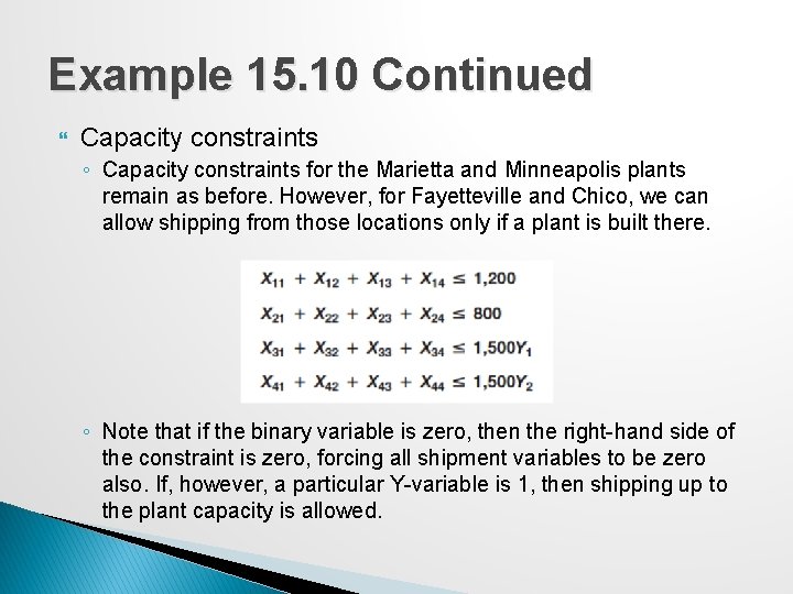
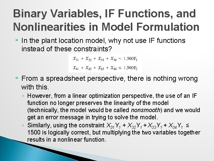
Example 15. 10 Continued Capacity constraints ◦ Capacity constraints for the Marietta and Minneapolis plants remain as before. However, for Fayetteville and Chico, we can allow shipping from those locations only if a plant is built there. ◦ Note that if the binary variable is zero, then the right-hand side of the constraint is zero, forcing all shipment variables to be zero also. If, however, a particular Y-variable is 1, then shipping up to the plant capacity is allowed.

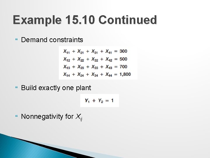
Example 15. 10 Continued Demand constraints Build exactly one plant Nonnegativity for Xij

Spreadsheet Model

Solver Model

Binary Variables, IF Functions, and Nonlinearities in Model Formulation In the plant location model, why not use IF functions instead of these constraints? From a spreadsheet perspective, there is nothing wrong with this. ◦ However, from a linear optimization perspective, the use of an IF function no longer preserves the linearity of the model (technically, the model would be called nonsmooth) and we would get an error message in trying to solve the model. ◦ Similarly, using the constraint X 31 Y 1 + X 32 Y 1 + X 33 Y 1 + X 34 Y 1 ≤ 1500 is logically correct, but multiplying the two variables together results in a nonlinear function.

Fixed-Cost Models Many business problems involve fixed costs; they are either incurred in full or not at all. Binary variables can be used to model such problems in a similar fashion as we did for the plant location model.

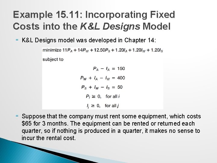
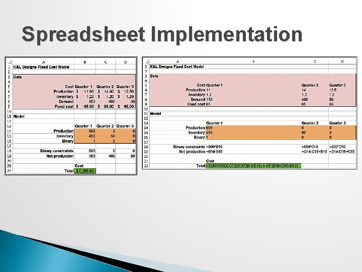
Example 15. 11: Incorporating Fixed Costs into the K&L Designs Model K&L Designs model was developed in Chapter 14: Suppose that the company must rent some equipment, which costs $65 for 3 months. The equipment can be rented or returned each quarter, so if nothing is produced in a quarter, it makes no sense to incur the rental cost.

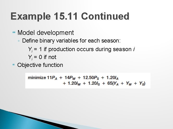
Example 15. 11 Continued Model development ◦ Define binary variables for each season: Yi = 1 if production occurs during season i Yi = 0 if not Objective function

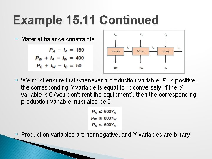
Example 15. 11 Continued Material balance constraints We must ensure that whenever a production variable, P, is positive, the corresponding Y variable is equal to 1; conversely, if the Y variable is 0 (you don’t rent the equipment), then the corresponding production variable must also be 0. Production variables are nonnegative, and Y variables are binary

Spreadsheet Implementation

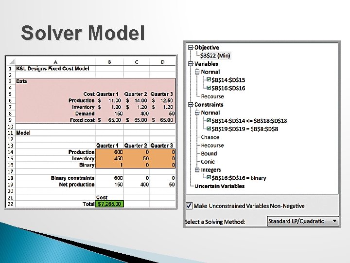
Solver Model

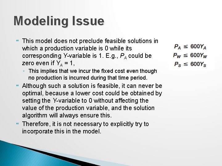
Modeling Issue This model does not preclude feasible solutions in which a production variable is 0 while its corresponding Y-variable is 1. E. g. , PA could be zero even if YA = 1, ◦ This implies that we incur the fixed cost even though no production is incurred during that time period. Although such a solution is feasible, it can never be optimal, because a lower cost could be obtained by setting the Y-variable to 0 without affecting the value of the production variable, and the solution algorithm will always ensure this. Therefore, it is not necessary to explicitly try to incorporate this in the model.