Inferences On Two Samples Overview We continue with

Inferences On Two Samples

Overview • We continue with confidence intervals and hypothesis testing for more advanced models • Models comparing two means – When the two means are dependent – When the two means are independent • Models comparing two proportions

Inference about Two Means: Dependent/paired Samples

Learning Objectives • Distinguish between independent and dependent sampling • Test hypotheses made regarding matchedpairs data • Construct and interpret confidence intervals about the population mean difference of matched-pairs data

Two populations • So far, we have covered a variety of models dealing with one population – The mean parameter for one population – The proportion parameter for one population • However, there are many real-world applications that need techniques to compare two populations

Examples • Examples of situations with two populations – We want to test whether a certain treatment helps or not … the measurements are the “before” measurement and the “after” measurement – We want to test the effectiveness of Drug A versus Drug B … we give 40 patients Drug A and 40 patients Drug B … the measurements are the Drug A and Drug B responses

Dependent Sample • In certain cases, the two samples are very closely tied to each other • A dependent sample is one when each individual in the first sample is directly matched to one individual in the second • Examples – Before and after measurements (a specific person’s before and the same person’s after) – Experiments on identical twins (twins matched with each other

Independent Sample • On the other extreme, the two samples can be completely independent of each other • An independent sample is when individuals selected for one sample have no relationship to the individuals selected for the other • Examples – Fifty samples from one factory compared to fifty samples from another – Two hundred patients divided at random into two groups of one hundred

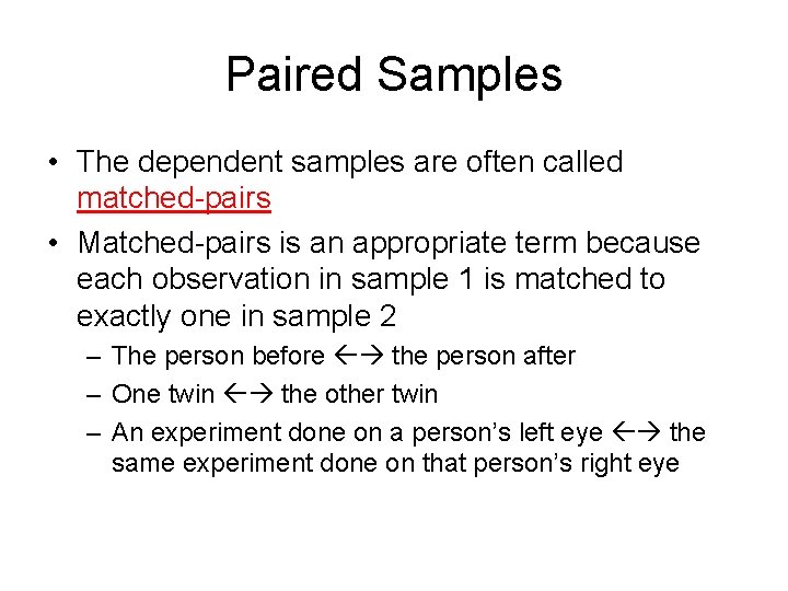
Paired Samples • The dependent samples are often called matched-pairs • Matched-pairs is an appropriate term because each observation in sample 1 is matched to exactly one in sample 2 – The person before the person after – One twin the other twin – An experiment done on a person’s left eye the same experiment done on that person’s right eye

Test hypotheses made regarding matched-pairs sample

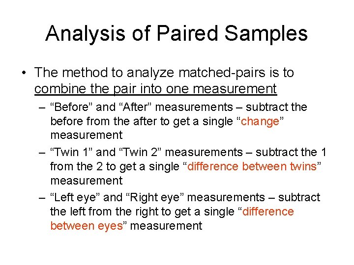
Analysis of Paired Samples • The method to analyze matched-pairs is to combine the pair into one measurement – “Before” and “After” measurements – subtract the before from the after to get a single “change” measurement – “Twin 1” and “Twin 2” measurements – subtract the 1 from the 2 to get a single “difference between twins” measurement – “Left eye” and “Right eye” measurements – subtract the left from the right to get a single “difference between eyes” measurement

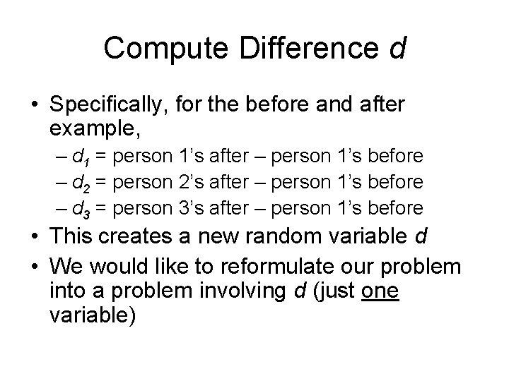
Compute Difference d • Specifically, for the before and after example, – d 1 = person 1’s after – person 1’s before – d 2 = person 2’s after – person 1’s before – d 3 = person 3’s after – person 1’s before • This creates a new random variable d • We would like to reformulate our problem into a problem involving d (just one variable)

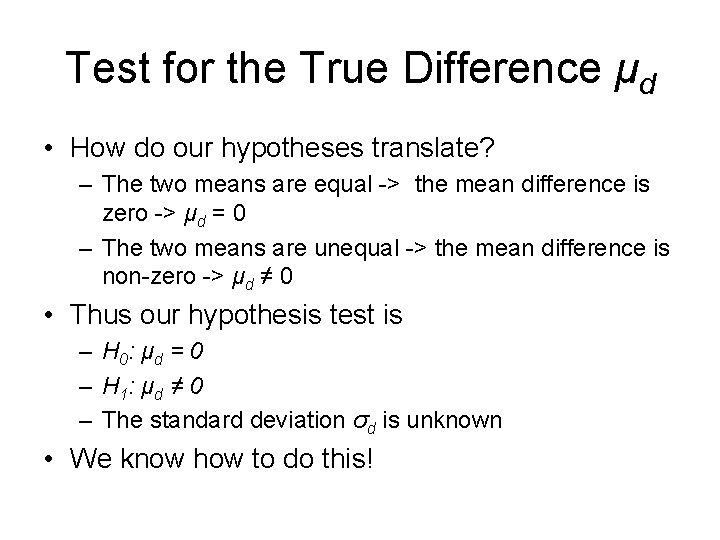
Test for the True Difference μd • How do our hypotheses translate? – The two means are equal -> the mean difference is zero -> μd = 0 – The two means are unequal -> the mean difference is non-zero -> μd ≠ 0 • Thus our hypothesis test is – H 0: μ d = 0 – H 1: μ d ≠ 0 – The standard deviation σd is unknown • We know how to do this!

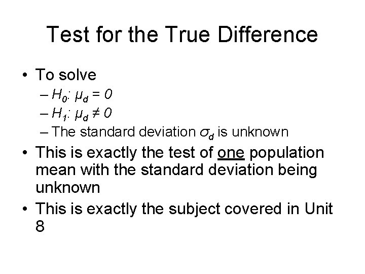
Test for the True Difference • To solve – H 0: μ d = 0 – H 1: μ d ≠ 0 – The standard deviation σd is unknown • This is exactly the test of one population mean with the standard deviation being unknown • This is exactly the subject covered in Unit 8

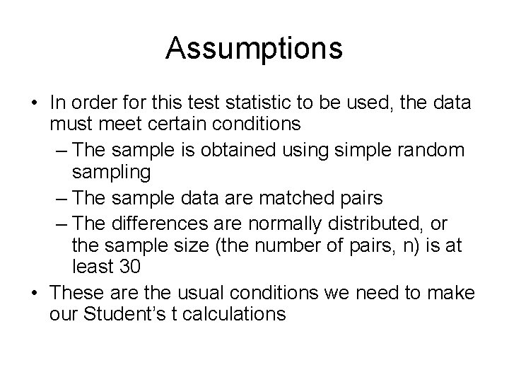
Assumptions • In order for this test statistic to be used, the data must meet certain conditions – The sample is obtained using simple random sampling – The sample data are matched pairs – The differences are normally distributed, or the sample size (the number of pairs, n) is at least 30 • These are the usual conditions we need to make our Student’s t calculations

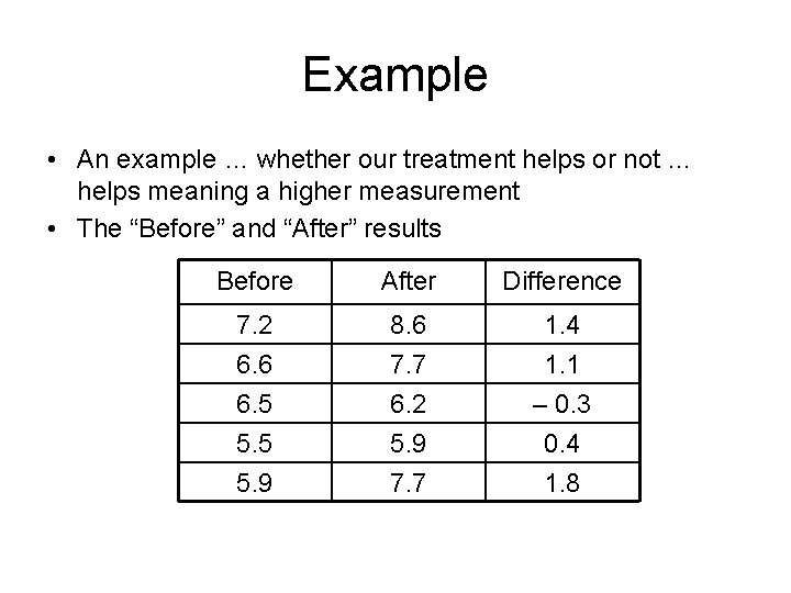
Example • An example … whether our treatment helps or not … helps meaning a higher measurement • The “Before” and “After” results Before After Difference 7. 2 6. 6 6. 5 8. 6 7. 7 6. 2 1. 4 1. 1 – 0. 3 5. 5 5. 9 7. 7 0. 4 1. 8

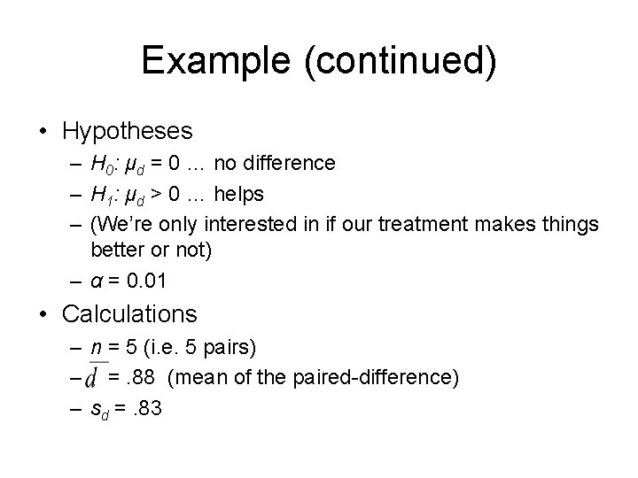
Example (continued) • Hypotheses – H 0: μd = 0 … no difference – H 1: μd > 0 … helps – (We’re only interested in if our treatment makes things better or not) – α = 0. 01 • Calculations – n = 5 (i. e. 5 pairs) – =. 88 (mean of the paired-difference) – sd =. 83

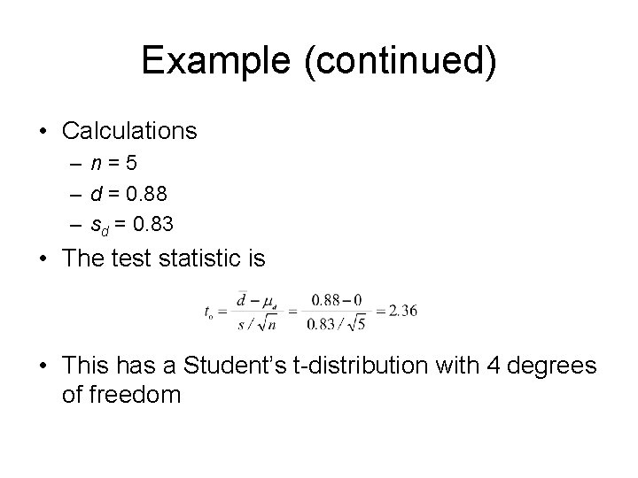
Example (continued) • Calculations – n=5 – d = 0. 88 – sd = 0. 83 • The test statistic is • This has a Student’s t-distribution with 4 degrees of freedom

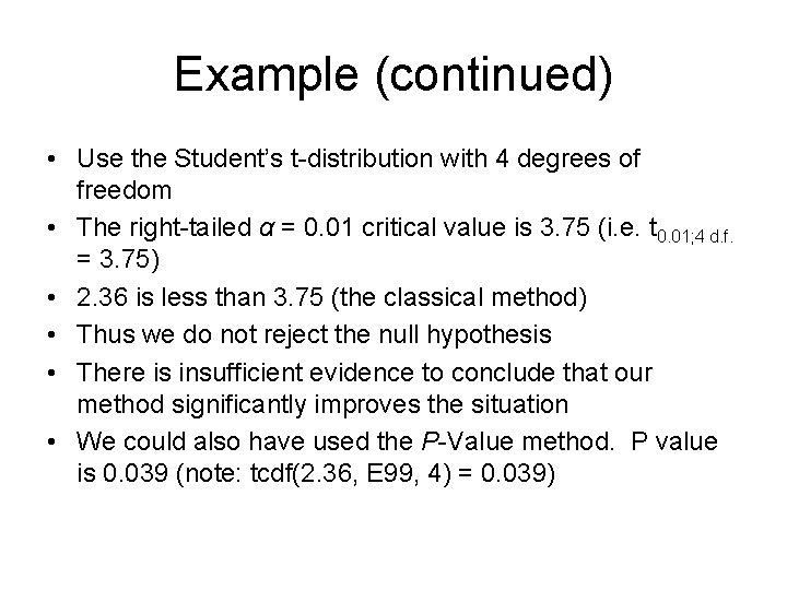
Example (continued) • Use the Student’s t-distribution with 4 degrees of freedom • The right-tailed α = 0. 01 critical value is 3. 75 (i. e. t 0. 01; 4 d. f. = 3. 75) • 2. 36 is less than 3. 75 (the classical method) • Thus we do not reject the null hypothesis • There is insufficient evidence to conclude that our method significantly improves the situation • We could also have used the P-Value method. P value is 0. 039 (note: tcdf(2. 36, E 99, 4) = 0. 039)

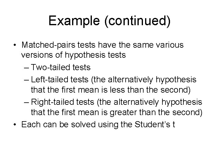
Example (continued) • Matched-pairs tests have the same various versions of hypothesis tests – Two-tailed tests – Left-tailed tests (the alternatively hypothesis that the first mean is less than the second) – Right-tailed tests (the alternatively hypothesis that the first mean is greater than the second) • Each can be solved using the Student’s t

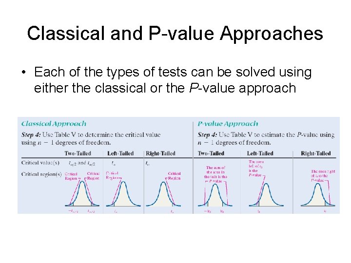
Classical and P-value Approaches • Each of the types of tests can be solved using either the classical or the P-value approach

Summary of the Method • A summary of the method – For each matched pair, subtract the first observation from the second – This results in one data item per subject with the data items independent of each other – Test that the mean of these differences is equal to 0 • Conclusions – Do not reject that μd = 0 – Reject that μd = 0. . . Reject that the two populations have the same mean

Construct and interpret confidence intervals about the population mean difference of matched-pairs data

Confidence Interval for the Paired Difference • We’ve turned the matched-pairs problem in one for a single variable’s mean / unknown standard deviation – We just did hypothesis tests – We can use the techniques taught in Unit 7 (again, single variable’s mean / unknown standard deviation) to construct confidence intervals • The idea – the processes (but maybe not the specific calculations) are very similar for all the different models

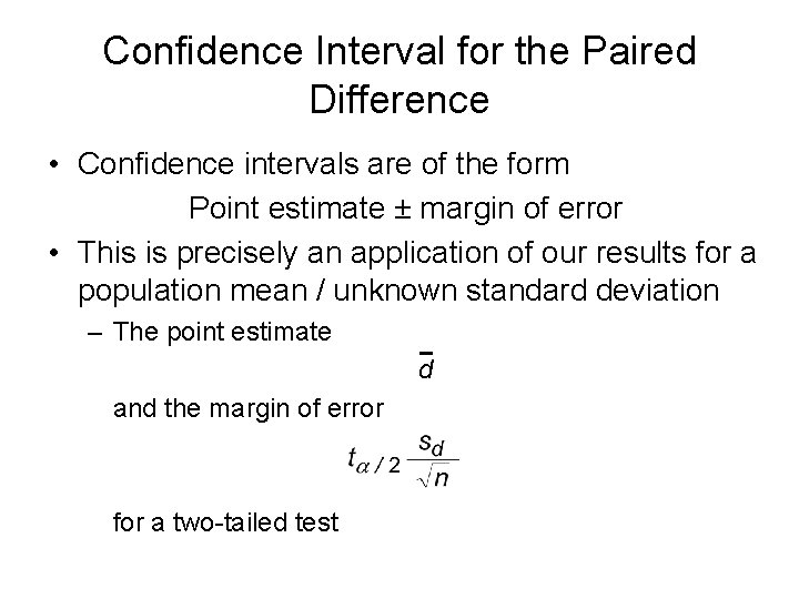
Confidence Interval for the Paired Difference • Confidence intervals are of the form Point estimate ± margin of error • This is precisely an application of our results for a population mean / unknown standard deviation – The point estimate d and the margin of error for a two-tailed test

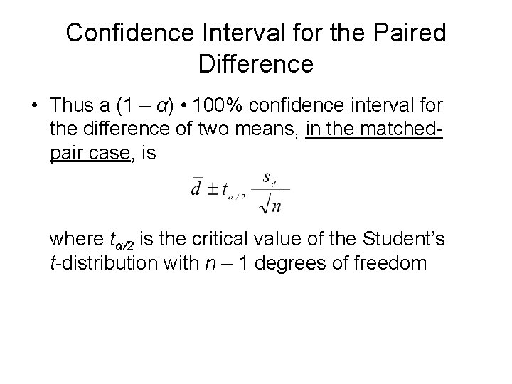
Confidence Interval for the Paired Difference • Thus a (1 – α) • 100% confidence interval for the difference of two means, in the matchedpair case, is where tα/2 is the critical value of the Student’s t-distribution with n – 1 degrees of freedom

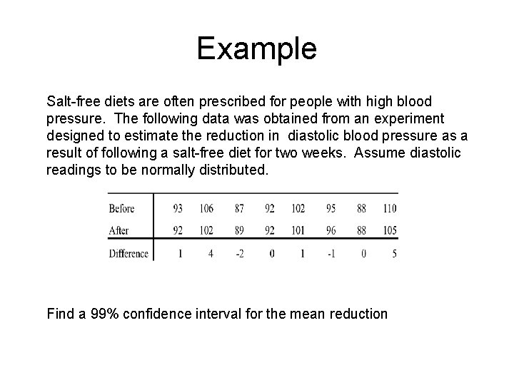
Example Salt-free diets are often prescribed for people with high blood pressure. The following data was obtained from an experiment designed to estimate the reduction in diastolic blood pressure as a result of following a salt-free diet for two weeks. Assume diastolic readings to be normally distributed. Find a 99% confidence interval for the mean reduction

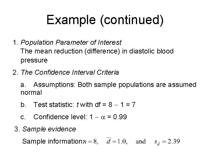
Example (continued) 1. Population Parameter of Interest The mean reduction (difference) in diastolic blood pressure 2. The Confidence Interval Criteria a. Assumptions: Both sample populations are assumed normal b. Test statistic: t with df = 8 - 1 = 7 c. Confidence level: 1 - a = 0. 99 3. Sample evidence Sample information:

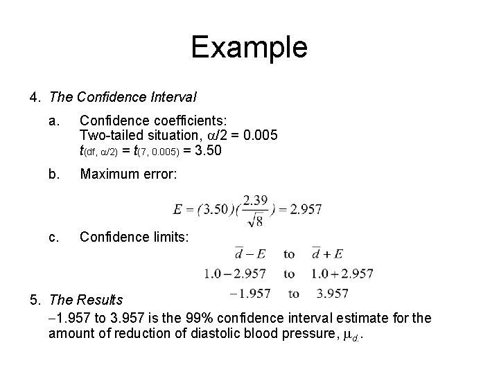
Example 4. The Confidence Interval a. Confidence coefficients: Two-tailed situation, a/2 = 0. 005 t(df, a/2) = t(7, 0. 005) = 3. 50 b. Maximum error: c. Confidence limits: 5. The Results -1. 957 to 3. 957 is the 99% confidence interval estimate for the amount of reduction of diastolic blood pressure, md. .

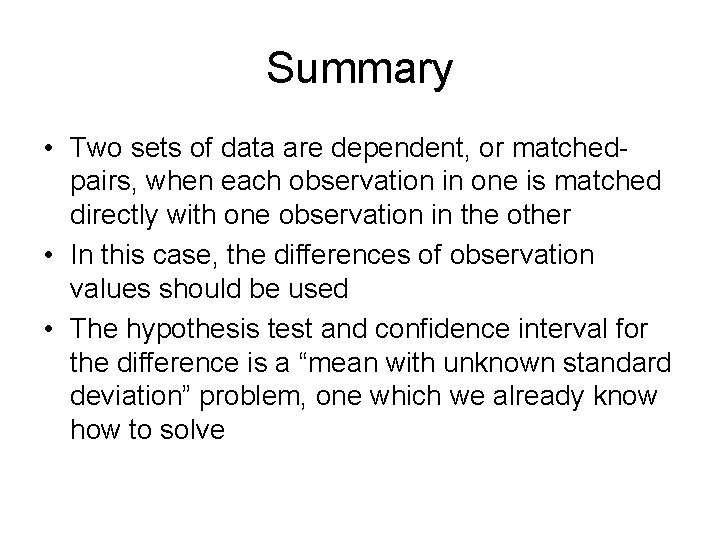
Summary • Two sets of data are dependent, or matchedpairs, when each observation in one is matched directly with one observation in the other • In this case, the differences of observation values should be used • The hypothesis test and confidence interval for the difference is a “mean with unknown standard deviation” problem, one which we already know how to solve

Inference about Two Means: Independent Samples

Learning Objectives • Test hypotheses regarding the difference of two independent means • Construct and interpret confidence intervals regarding the difference of two independent means

Independent Samples • Two samples are independent if the values in one have no relation to the values in the other • Examples of not independent – Data from male students versus data from business majors (an overlap in populations) – The mean amount of rain, per day, reported in two weather stations in neighboring towns (likely to rain in both places)

Independent Samples • A typical example of an independent samples test is to test whether a new drug, Drug N, lowers cholesterol levels more than the current drug, Drug C • A group of 100 patients could be chosen – The group could be divided into two groups of 50 using a random method – If we use a random method (such as a simple random sample of 50 out of the 100 patients), then the two groups would be independent

Test of Two Independent Samples • The test of two independent samples is very similar, in process, to the test of a single population mean • The only major difference is that a different test statistic is used • We will discuss the new test statistic through an analogy with the hypothesis test of one mean

Test hypotheses regarding the difference of two independent means

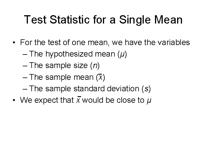
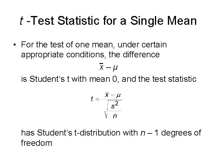
Test Statistic for a Single Mean • For the test of one mean, we have the variables – The hypothesized mean (μ) – The sample size (n) – The sample mean (x) – The sample standard deviation (s) • We expect that x would be close to μ

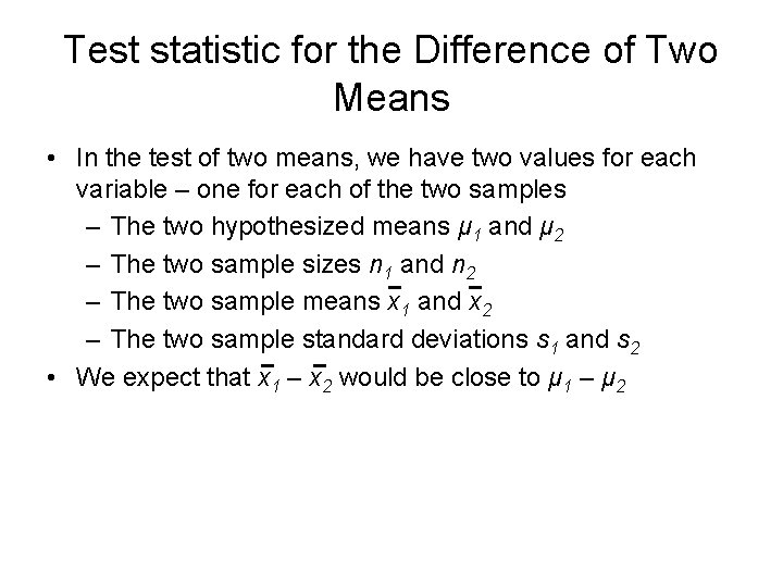
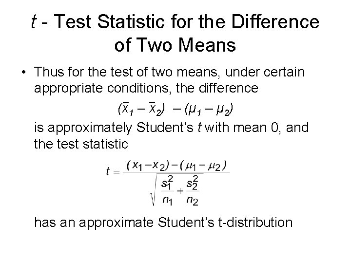
Test statistic for the Difference of Two Means • In the test of two means, we have two values for each variable – one for each of the two samples – The two hypothesized means μ 1 and μ 2 – The two sample sizes n 1 and n 2 – The two sample means x 1 and x 2 – The two sample standard deviations s 1 and s 2 • We expect that x 1 – x 2 would be close to μ 1 – μ 2

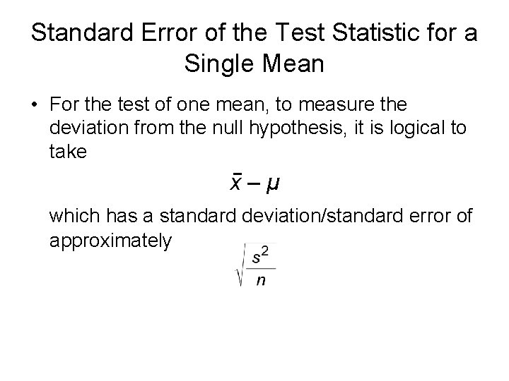
Standard Error of the Test Statistic for a Single Mean • For the test of one mean, to measure the deviation from the null hypothesis, it is logical to take x–μ which has a standard deviation/standard error of approximately

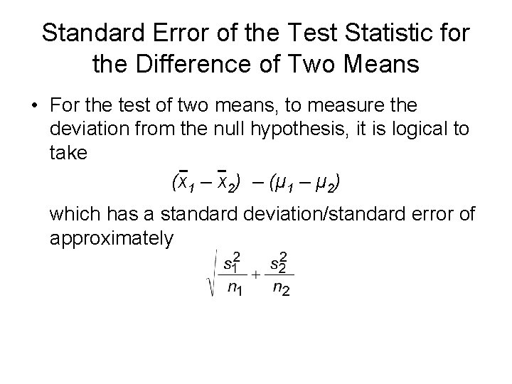
Standard Error of the Test Statistic for the Difference of Two Means • For the test of two means, to measure the deviation from the null hypothesis, it is logical to take (x 1 – x 2) – (μ 1 – μ 2) which has a standard deviation/standard error of approximately

t -Test Statistic for a Single Mean • For the test of one mean, under certain appropriate conditions, the difference x–μ is Student’s t with mean 0, and the test statistic has Student’s t-distribution with n – 1 degrees of freedom

t - Test Statistic for the Difference of Two Means • Thus for the test of two means, under certain appropriate conditions, the difference (x 1 – x 2) – (μ 1 – μ 2) is approximately Student’s t with mean 0, and the test statistic has an approximate Student’s t-distribution

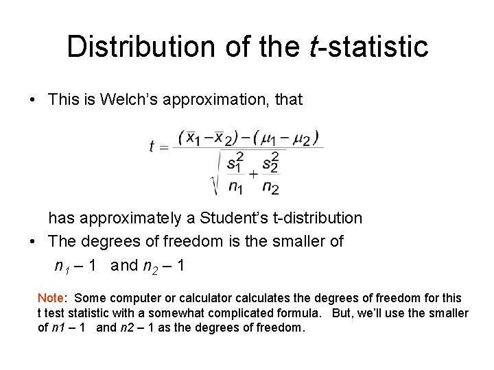
Distribution of the t-statistic • This is Welch’s approximation, that has approximately a Student’s t-distribution • The degrees of freedom is the smaller of n 1 – 1 and n 2 – 1 Note: Some computer or calculates the degrees of freedom for this t test statistic with a somewhat complicated formula. But, we’ll use the smaller of n 1 – 1 and n 2 – 1 as the degrees of freedom.

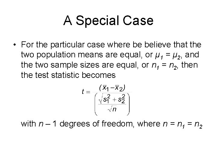
A Special Case • For the particular case where be believe that the two population means are equal, or μ 1 = μ 2, and the two sample sizes are equal, or n 1 = n 2, then the test statistic becomes with n – 1 degrees of freedom, where n = n 1 = n 2

General Test Procedure • Now for the overall structure of the test – Set up the hypotheses – Select the level of significance α – Compute the test statistic – Compare the test statistic with the appropriate critical values – Reach a do not reject or reject the null hypothesis conclusion

Assumptions • In order for this method to be used, the data must meet certain conditions – Both samples are obtained using simple random sampling – The samples are independent – The populations are normally distributed, or the sample sizes are large (both n 1 and n 2 are at least 30) • These are the usual conditions we need to make our Student’s t calculations

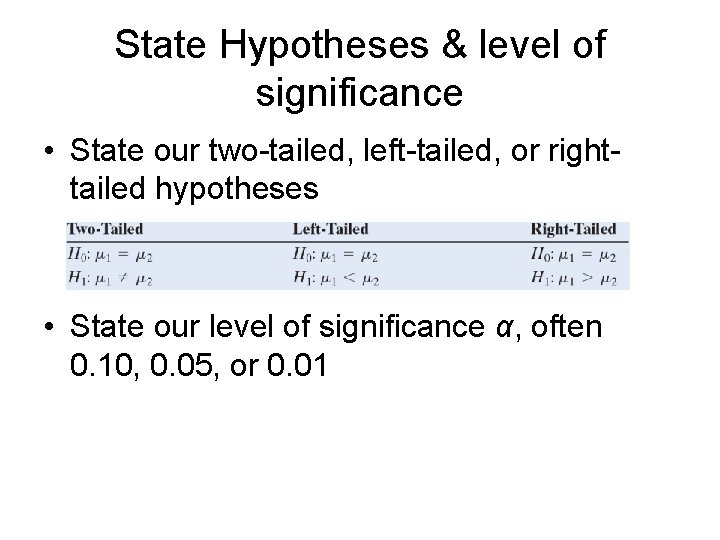
State Hypotheses & level of significance • State our two-tailed, left-tailed, or righttailed hypotheses • State our level of significance α, often 0. 10, 0. 05, or 0. 01

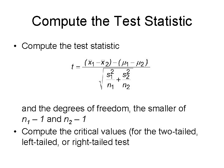
Compute the Test Statistic • Compute the test statistic and the degrees of freedom, the smaller of n 1 – 1 and n 2 – 1 • Compute the critical values (for the two-tailed, left-tailed, or right-tailed test

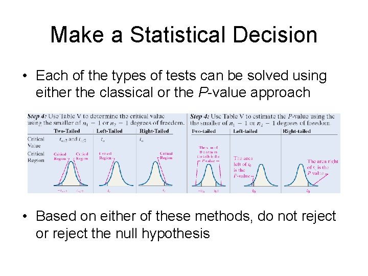
Make a Statistical Decision • Each of the types of tests can be solved using either the classical or the P-value approach • Based on either of these methods, do not reject or reject the null hypothesis

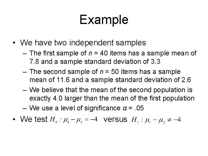
Example • We have two independent samples – The first sample of n = 40 items has a sample mean of 7. 8 and a sample standard deviation of 3. 3 – The second sample of n = 50 items has a sample mean of 11. 6 and a sample standard deviation of 2. 6 – We believe that the mean of the second population is exactly 4. 0 larger than the mean of the first population – We use a level of significance α =. 05 • We test versus

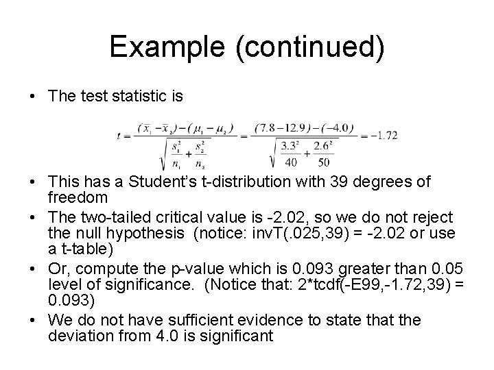
Example (continued) • The test statistic is • This has a Student’s t-distribution with 39 degrees of freedom • The two-tailed critical value is -2. 02, so we do not reject the null hypothesis (notice: inv. T(. 025, 39) = -2. 02 or use a t-table) • Or, compute the p-value which is 0. 093 greater than 0. 05 level of significance. (Notice that: 2*tcdf(-E 99, -1. 72, 39) = 0. 093) • We do not have sufficient evidence to state that the deviation from 4. 0 is significant

Construct and interpret confidence intervals regarding the difference of two independent means

Confidence Interval of m 1 -m 2 • Confidence intervals are of the form Point estimate ± margin of error • We can compare our confidence interval with the test statistic from our hypothesis test – The point estimate is x 1 – x 2 – We use the denominator of the test statistic as the standard error – We use critical values from the Student’s t

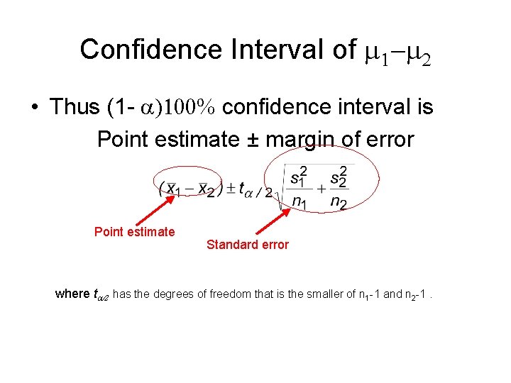
Confidence Interval of m 1 -m 2 • Thus (1 - a)100% confidence interval is Point estimate ± margin of error Point estimate Standard error where ta/2 has the degrees of freedom that is the smaller of n 1 -1 and n 2 -1.

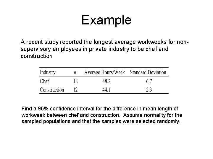
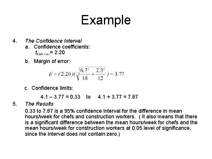
Example A recent study reported the longest average workweeks for nonsupervisory employees in private industry to be chef and construction Find a 95% confidence interval for the difference in mean length of workweek between chef and construction. Assume normality for the sampled populations and that the samples were selected randomly.

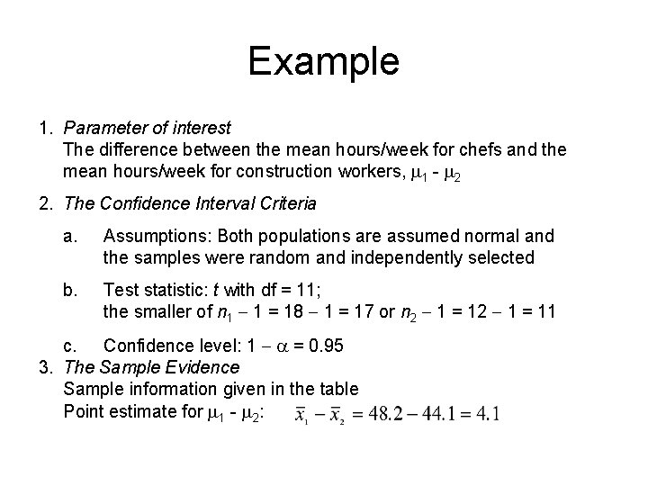
Example 1. Parameter of interest The difference between the mean hours/week for chefs and the mean hours/week for construction workers, m 1 - m 2 2. The Confidence Interval Criteria a. Assumptions: Both populations are assumed normal and the samples were random and independently selected b. Test statistic: t with df = 11; the smaller of n 1 - 1 = 18 - 1 = 17 or n 2 - 1 = 11 c. Confidence level: 1 - a = 0. 95 3. The Sample Evidence Sample information given in the table Point estimate for m 1 - m 2:

Example 4. The Confidence Interval a. Confidence coefficients: t 0. 025, 11 d. f. = 2. 20 b. Margin of error: c. Confidence limits: 5. 4. 1 – 3. 77 = 0. 33 to 4. 1 + 3. 77 = 7. 87 The Results 0. 33 to 7. 87 is a 95% confidence interval for the difference in mean hours/week for chefs and construction workers. ( It also means that there is a significant difference between the mean hours/week for chefs and the mean hours/week for construction workers at 0. 05 level of significance, since the interval does not contain zero. )

Summary • Two sets of data are independent when observations in one have no affect on observations in the other • In this case, the differences of the two means should be used in a Student’s t-test • The overall process, other than the formula for the standard error, are the general hypothesis test and confidence intervals process

Inference about Two Population Proportions

Learning Objectives • Test hypotheses regarding two population proportions • Construct and interpret confidence intervals for the difference between two population proportions

Test hypotheses regarding two population proportions

Inference about Two Proportions • This progression should not be a surprise • One mean and one proportion – Unit 7 – confidence intervals – Unit 8 – hypothesis tests • Two means – Unit 9 - hypothesis tests and confidence intervals • Now for two proportions …

Examples • We now compare two proportions, testing whether they are the same or not • Examples – The proportion of women (population one) who have a certain trait versus the proportion of men (population two) who have that same trait – The proportion of white sheep (population one) who have a certain characteristic versus the proportion of black sheep (population two) who have that same characteristic

Two Population Proportions • The test of two populations proportions is very similar, in process, to the test of one population proportion and the test of two population means • The only major difference is that a different test statistic is used • We will discuss the new test statistic through an analogy with the hypothesis test of one proportion

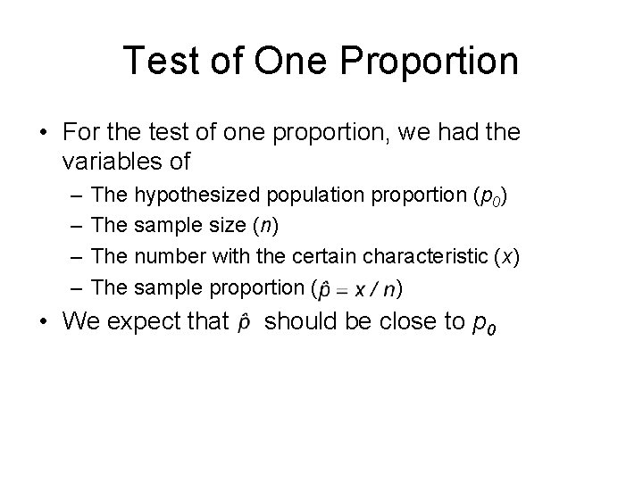
Test of One Proportion • For the test of one proportion, we had the variables of – – The hypothesized population proportion (p 0) The sample size (n) The number with the certain characteristic (x) The sample proportion ( ) • We expect that should be close to p 0

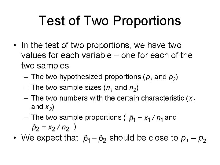
Test of Two Proportions • In the test of two proportions, we have two values for each variable – one for each of the two samples – The two hypothesized proportions (p 1 and p 2) – The two sample sizes (n 1 and n 2) – The two numbers with the certain characteristic (x 1 and x 2) – The two sample proportions ( and ) • We expect that should be close to p 1 – p 2

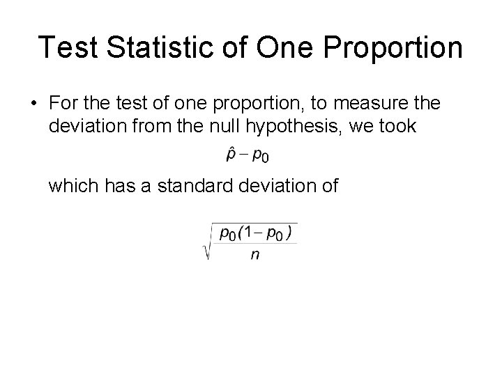
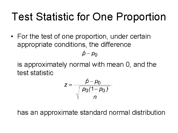
Test Statistic of One Proportion • For the test of one proportion, to measure the deviation from the null hypothesis, we took which has a standard deviation of

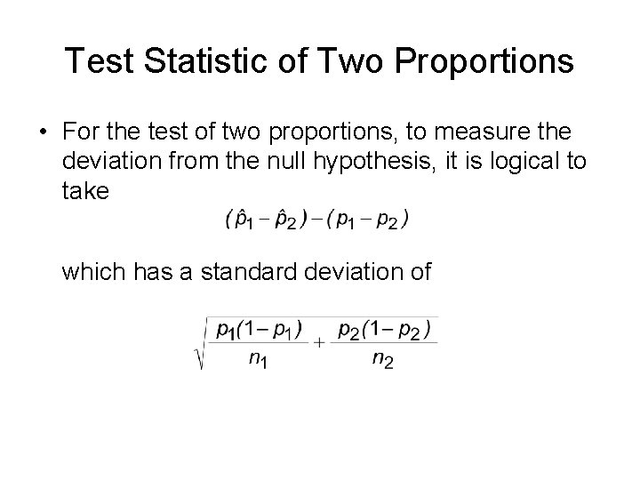
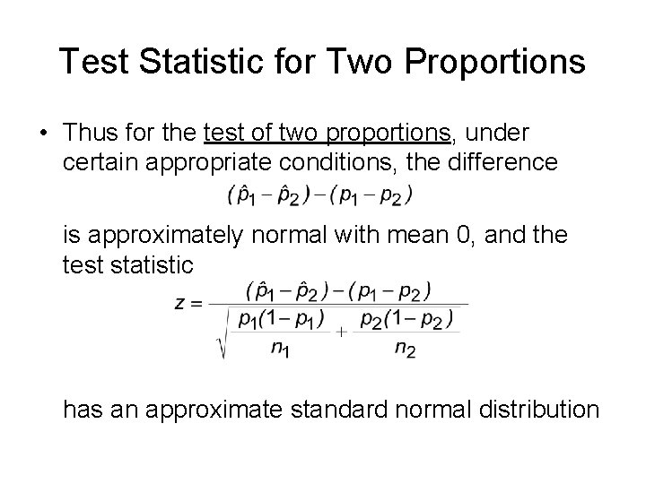
Test Statistic of Two Proportions • For the test of two proportions, to measure the deviation from the null hypothesis, it is logical to take which has a standard deviation of

Test Statistic for One Proportion • For the test of one proportion, under certain appropriate conditions, the difference is approximately normal with mean 0, and the test statistic has an approximate standard normal distribution

Test Statistic for Two Proportions • Thus for the test of two proportions, under certain appropriate conditions, the difference is approximately normal with mean 0, and the test statistic has an approximate standard normal distribution

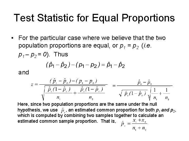
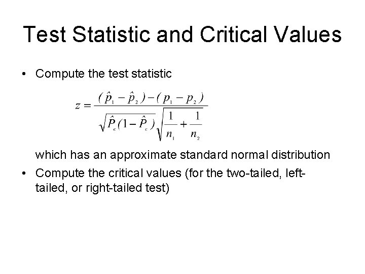
Test Statistic for Equal Proportions • For the particular case where we believe that the two population proportions are equal, or p 1 = p 2 (i. e. p 1 – p 2 = 0). Thus and Here, since two population proportions are the same under the null hypothesis, we use , an estimated common proportion for both p 1 and p 2, which is computed by combining two samples together to calculate an estimated common sample proportion. That is,

General Test Procedure • Now for the overall structure of the test – Set up the hypotheses – Select the level of significance α – Compute the test statistic – Compare the test statistic with the appropriate critical values – Reach a do not reject or reject the null hypothesis conclusion

Assumptions • In order for this method to be used, the data must meet certain conditions – Both samples are obtained independently using simple random sampling – Each sample size is large • These are the usual conditions we need to make our test of proportions calculations

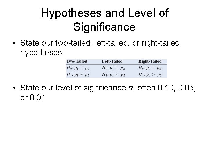
Hypotheses and Level of Significance • State our two-tailed, left-tailed, or right-tailed hypotheses • State our level of significance α, often 0. 10, 0. 05, or 0. 01

Test Statistic and Critical Values • Compute the test statistic which has an approximate standard normal distribution • Compute the critical values (for the two-tailed, lefttailed, or right-tailed test)

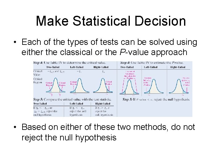
Make Statistical Decision • Each of the types of tests can be solved using either the classical or the P-value approach • Based on either of these two methods, do not reject the null hypothesis

Example • We have two independent samples – 55 out of a random sample of 100 students at one university are commuters – 80 out of a random sample of 200 students at another university are commuters – We wish to know of these two proportions are equal – We use a level of significance α =. 05 • Both samples sizes are large so our method can be used

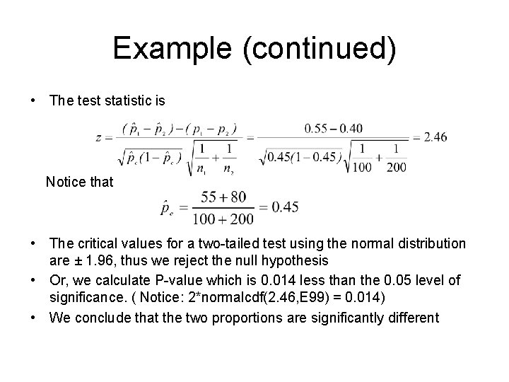
Example (continued) • The test statistic is Notice that • The critical values for a two-tailed test using the normal distribution are ± 1. 96, thus we reject the null hypothesis • Or, we calculate P-value which is 0. 014 less than the 0. 05 level of significance. ( Notice: 2*normalcdf(2. 46, E 99) = 0. 014) • We conclude that the two proportions are significantly different

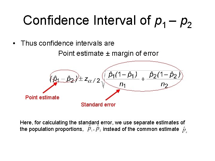
Confidence Interval of p 1 – p 2 • Thus confidence intervals are Point estimate ± margin of error Point estimate Standard error Here, for calculating the standard error, we use separate estimates of the population proportions, instead of the common estimate

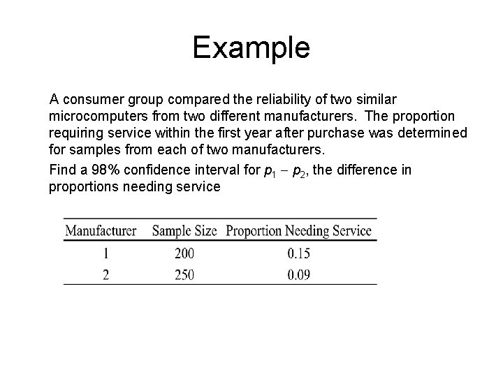
Example A consumer group compared the reliability of two similar microcomputers from two different manufacturers. The proportion requiring service within the first year after purchase was determined for samples from each of two manufacturers. Find a 98% confidence interval for p 1 - p 2, the difference in proportions needing service

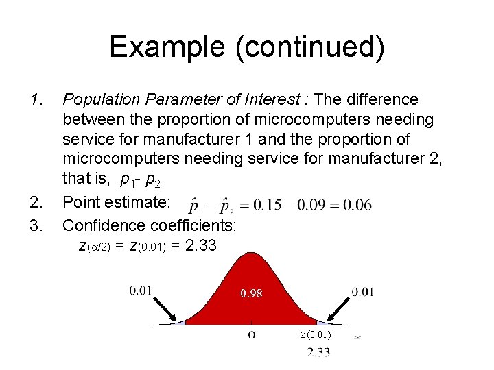
Example (continued) 1. 2. 3. Population Parameter of Interest : The difference between the proportion of microcomputers needing service for manufacturer 1 and the proportion of microcomputers needing service for manufacturer 2, that is, p 1 - p 2 Point estimate: Confidence coefficients: z(a/2) = z(0. 01) = 2. 33 0. 98 z(0. 01)

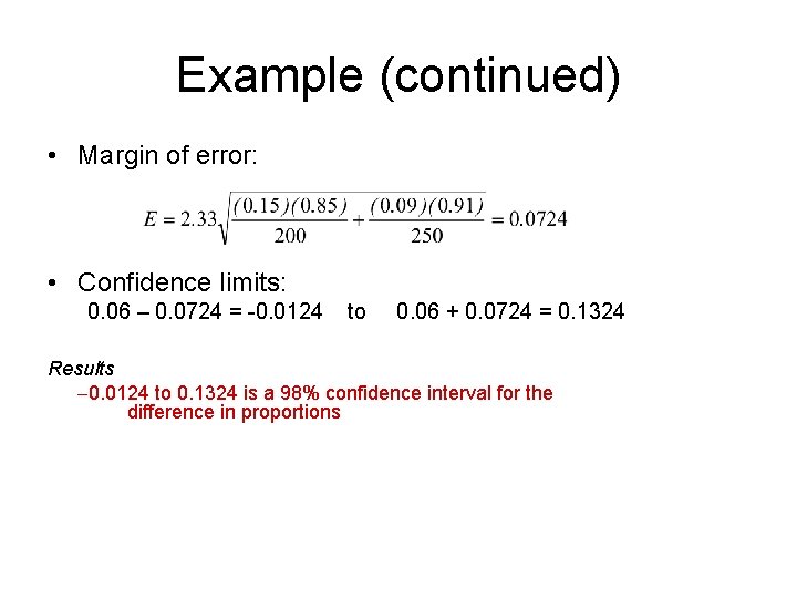
Example (continued) • Margin of error: • Confidence limits: 0. 06 – 0. 0724 = -0. 0124 to 0. 06 + 0. 0724 = 0. 1324 Results -0. 0124 to 0. 1324 is a 98% confidence interval for the difference in proportions

Summary • We can compare proportions from two independent samples • We use a formula with the combined sample sizes and proportions for the standard error • The overall process, other than the formula for the standard error, are the general hypothesis test and confidence intervals process

Inferences on Two Samples Summary

Summary • The process of hypothesis testing is very similar across the testing of different parameters • The major steps in hypothesis testing are – Formulate the appropriate null and alternative hypotheses – Calculate the test statistic – Determine the appropriate critical value or values – Reach the reject / do not reject conclusions

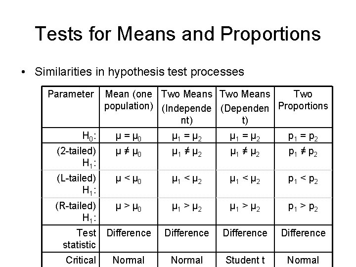
Tests for Means and Proportions • Similarities in hypothesis test processes Parameter Mean (one Two Means Two population) (Independe (Dependen Proportions nt) t) H 0 : μ = μ 0 μ 1 = μ 2 p 1 = p 2 (2 -tailed) H 1 : μ ≠ μ 0 μ 1 ≠ μ 2 p 1 ≠ p 2 (L-tailed) H 1 : μ < μ 0 μ 1 < μ 2 p 1 < p 2 (R-tailed) H 1 : μ > μ 0 μ 1 > μ 2 p 1 > p 2 Test statistic Difference Critical Normal Student t Normal

Summary • We can test whether sample data from two different samples supports a hypothesis claim about a population mean or proportion • For two population means, there are two cases – Dependent (or matched-pair) samples – Independent samples • All of these tests follow very similar processes, differing only in their test statistics and the distributions for their critical values