Inferences from Two samples Statistical Methods in Health

Inferences from Two samples Statistical Methods in Health Administration • By: - Abdalkarrem Fahad Alashjaai - Albaraa Abdullah Alhowaimil - Falah Salem Alqahtani 9. 1 - 1

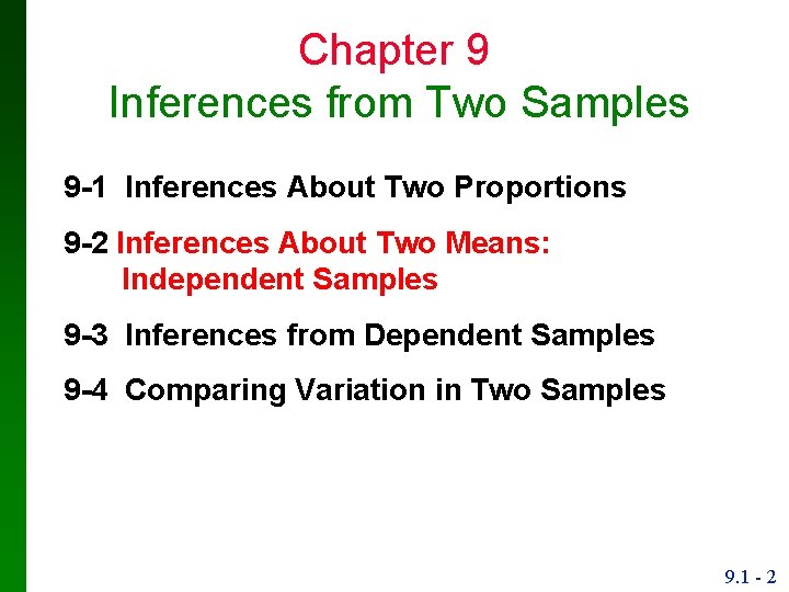
Chapter 9 Inferences from Two Samples 9 -1 Inferences About Two Proportions 9 -2 Inferences About Two Means: Independent Samples 9 -3 Inferences from Dependent Samples 9 -4 Comparing Variation in Two Samples 9. 1 - 2

Section 9 -3 Inferences About Two Means: Independent Samples 9. 1 - 3

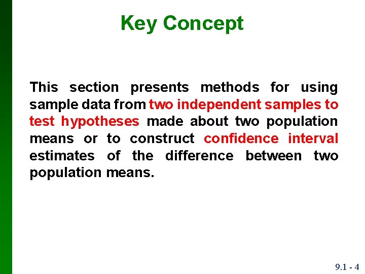
Key Concept This section presents methods for using sample data from two independent samples to test hypotheses made about two population means or to construct confidence interval estimates of the difference between two population means. 9. 1 - 4

Key Concept In Part 1 we discuss situations in which the standard deviations of the two populations are unknown and are not assumed to be equal. In Part 2 we discuss two other situations: (1) The two population standard deviations are both known; (2) the two population standard deviations are unknown but are assumed to be equal. Because is typically unknown in real situations, most attention should be given to the methods described in Part 1. 9. 1 - 5

Part 1: Independent Samples with σ1 and σ2 Unknown and Not Assumed Equal 9. 1 - 6

Definitions Two samples are independent if the sample values selected from one population are not related to or somehow paired or matched with the sample values from the other population. Two samples are dependent if the sample values are paired. (That is, each pair of sample values consists of two measurements from the same subject (such as before/after data), or each pair of sample values consists of matched pairs (such as husband/wife data), where the matching is based on some inherent relationship. ) 9. 1 - 7

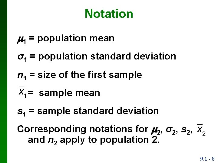
Notation 1 = population mean σ1 = population standard deviation n 1 = size of the first sample = sample mean s 1 = sample standard deviation Corresponding notations for 2, σ2, s 2, and n 2 apply to population 2. 9. 1 - 8

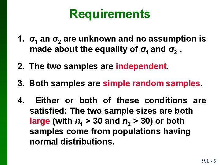
Requirements 1. σ1 an σ2 are unknown and no assumption is made about the equality of σ1 and σ2. 2. The two samples are independent. 3. Both samples are simple random samples. 4. Either or both of these conditions are satisfied: The two sample sizes are both large (with n 1 > 30 and n 2 > 30) or both samples come from populations having normal distributions. 9. 1 - 9

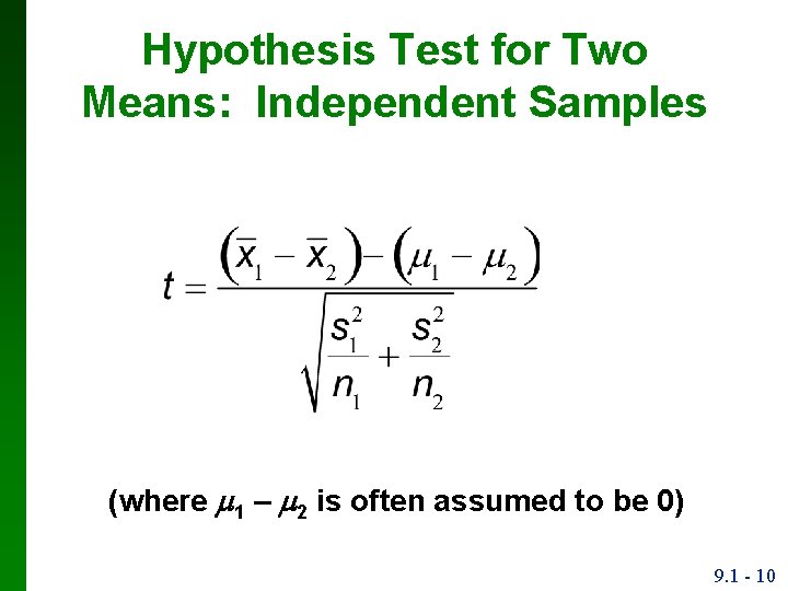
Hypothesis Test for Two Means: Independent Samples (where 1 – 2 is often assumed to be 0) 9. 1 - 10

Hypothesis Test - cont Test Statistic for Two Means: Independent Samples 9. 1 - 11

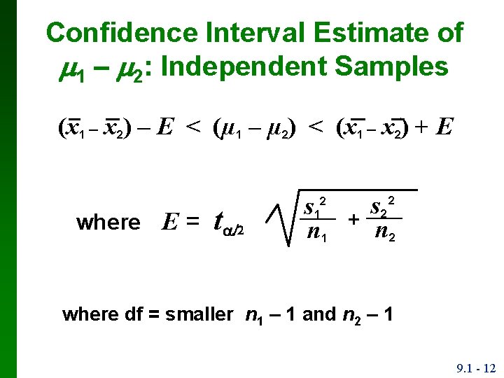
Confidence Interval Estimate of 1 – 2: Independent Samples (x 1 – x 2) – E < (µ 1 – µ 2) < (x 1 – x 2) + E where E = t s 2 s + n 2 n 1 2 where df = smaller n 1 – 1 and n 2 – 1 9. 1 - 12

Caution Before conducting a hypothesis test, consider the context of the data, the source of the data, the sampling method, and explore the data with graphs and descriptive statistics. Be sure to verify that the requirements are satisfied. 9. 1 - 13

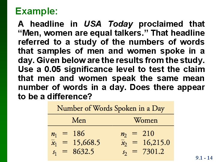
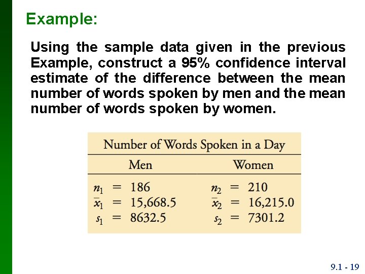
Example: A headline in USA Today proclaimed that “Men, women are equal talkers. ” That headline referred to a study of the numbers of words that samples of men and women spoke in a day. Given below are the results from the study. Use a 0. 05 significance level to test the claim that men and women speak the same mean number of words in a day. Does there appear to be a difference? 9. 1 - 14

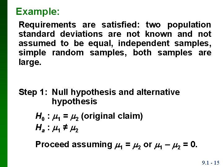
Example: Requirements are satisfied: two population standard deviations are not known and not assumed to be equal, independent samples, simple random samples, both samples are large. Step 1: Null hypothesis and alternative hypothesis H 0 : 1 = 2 (original claim) Ha : 1 ≠ 2 Proceed assuming 1 = 2 or 1 – 2 = 0. 9. 1 - 15

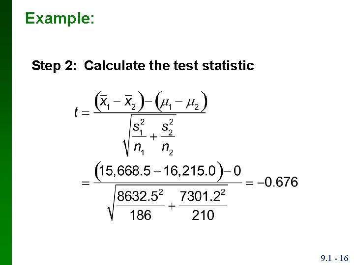
Example: Step 2: Calculate the test statistic 9. 1 - 16

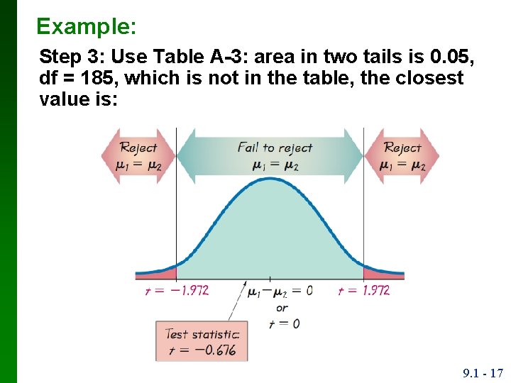
Example: Step 3: Use Table A-3: area in two tails is 0. 05, df = 185, which is not in the table, the closest value is: t = ± 1. 972 9. 1 - 17

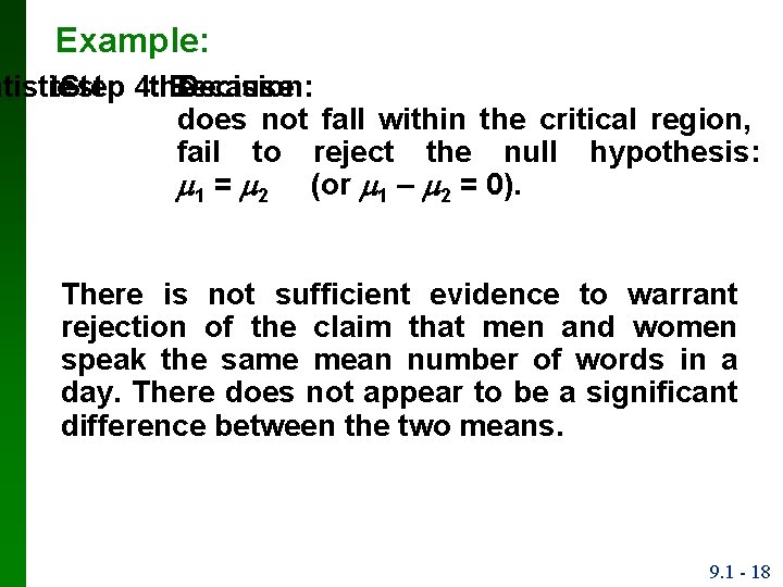
Example: atistic test Step 4: the Because Decision: does not fall within the critical region, fail to reject the null hypothesis: 1 = 2 (or 1 – 2 = 0). There is not sufficient evidence to warrant rejection of the claim that men and women speak the same mean number of words in a day. There does not appear to be a significant difference between the two means. 9. 1 - 18

Example: Using the sample data given in the previous Example, construct a 95% confidence interval estimate of the difference between the mean number of words spoken by men and the mean number of words spoken by women. 9. 1 - 19

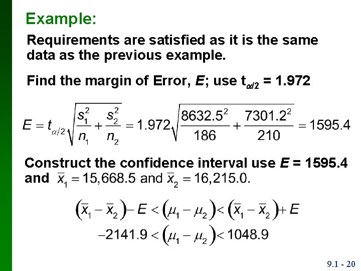
Example: Requirements are satisfied as it is the same data as the previous example. Find the margin of Error, E; use t /2 = 1. 972 Construct the confidence interval use E = 1595. 4 and 9. 1 - 20

Independent Samples with σ1 and σ2 Known. 9. 1 - 21

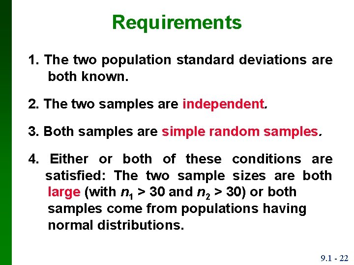
Requirements 1. The two population standard deviations are both known. 2. The two samples are independent. 3. Both samples are simple random samples. 4. Either or both of these conditions are satisfied: The two sample sizes are both large (with n 1 > 30 and n 2 > 30) or both samples come from populations having normal distributions. 9. 1 - 22

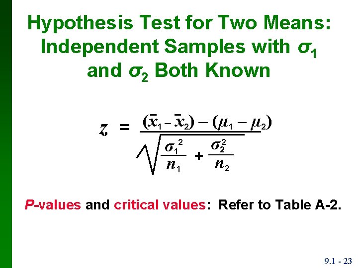
Hypothesis Test for Two Means: Independent Samples with σ1 and σ2 Both Known z (x 1 – x 2) – (µ 1 – µ 2) = 2 2 σ σ1 2 + n 2 n 1 P-values and critical values: Refer to Table A-2. 9. 1 - 23

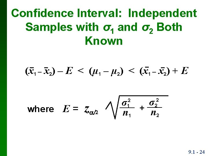
Confidence Interval: Independent Samples with σ1 and σ2 Both Known (x 1 – x 2) – E < (µ 1 – µ 2) < (x 1 – x 2) + E where E = z σ σ + n 2 n 1 2 2 9. 1 - 24

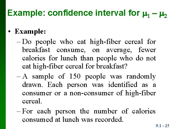
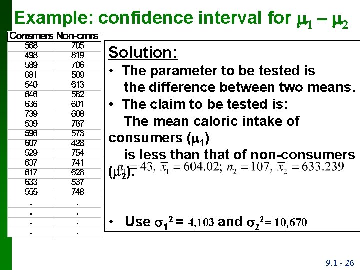
Example: confidence interval for m 1 – m • Example: – Do people who eat high-fiber cereal for breakfast consume, on average, fewer calories for lunch than people who do not eat high-fiber cereal for breakfast? – A sample of 150 people was randomly drawn. Each person was identified as a consumer or a non-consumer of high-fiber cereal. – For each person the number of calories consumed at lunch was recorded. 9. 1 - 25

Example: confidence interval for m 1 – m Solution: • The parameter to be tested is the difference between two means. • The claim to be tested is: The mean caloric intake of consumers (m 1) is less than that of non-consumers (m 2). • Use 12 = 4, 103 and 22= 10, 670 9. 1 - 26

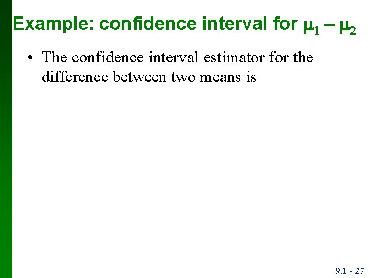
Example: confidence interval for m 1 – m • The confidence interval estimator for the difference between two means is 9. 1 - 27

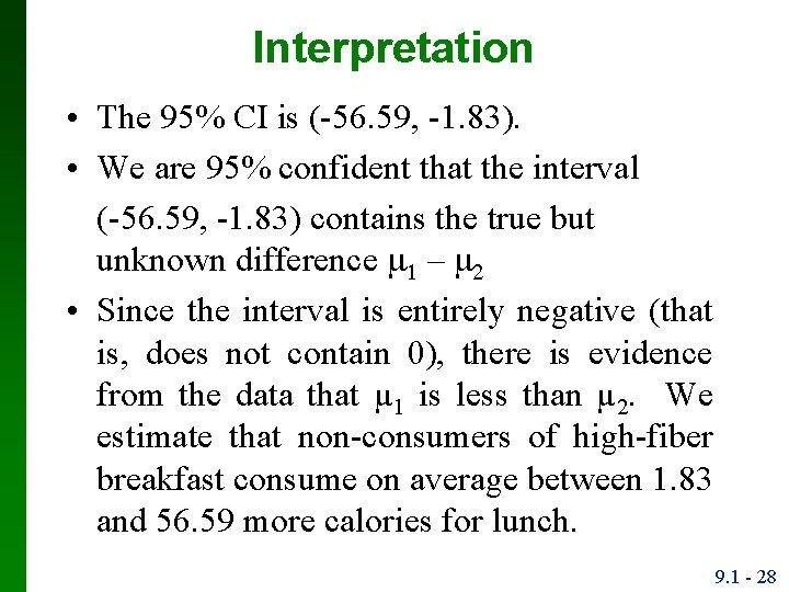
Interpretation • The 95% CI is (-56. 59, -1. 83). • We are 95% confident that the interval (-56. 59, -1. 83) contains the true but unknown difference m 1 – m 2 • Since the interval is entirely negative (that is, does not contain 0), there is evidence from the data that µ 1 is less than µ 2. We estimate that non-consumers of high-fiber breakfast consume on average between 1. 83 and 56. 59 more calories for lunch. 9. 1 - 28

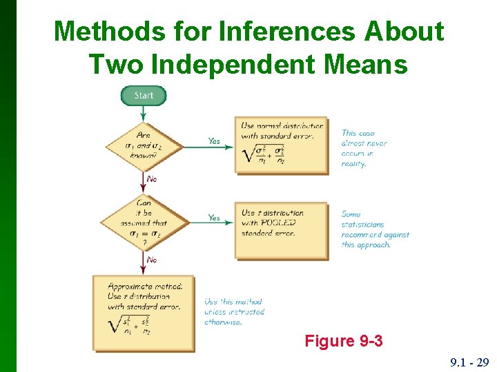
Methods for Inferences About Two Independent Means Figure 9 -3 9. 1 - 29

Assume that σ1 = σ2 and Pool the Sample Variances. 9. 1 - 30

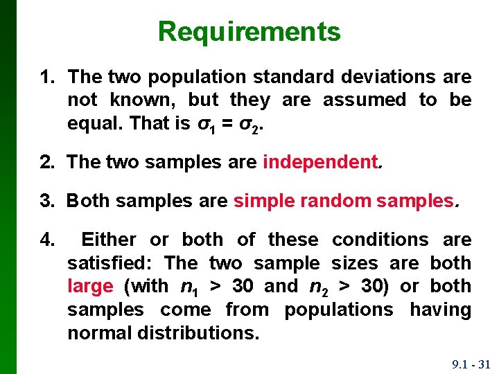
Requirements 1. The two population standard deviations are not known, but they are assumed to be equal. That is σ1 = σ2. 2. The two samples are independent. 3. Both samples are simple random samples. 4. Either or both of these conditions are satisfied: The two sample sizes are both large (with n 1 > 30 and n 2 > 30) or both samples come from populations having normal distributions. 9. 1 - 31

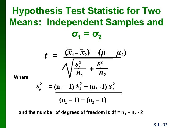
Hypothesis Test Statistic for Two Means: Independent Samples and σ1 = σ2 t Where s 2. p (x 1 – x 2) – (µ 1 – µ 2) = 2 2 s sp p + n 2 n 1 = (n 1 – 1) s + (n 2 -1) s 22 2 1 (n 1 – 1) + (n 2 – 1) and the number of degrees of freedom is df = n 1 + n 2 - 2 9. 1 - 32

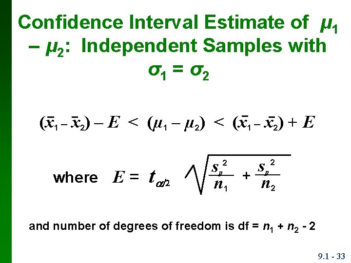
Confidence Interval Estimate of μ 1 – μ 2: Independent Samples with σ1 = σ2 (x 1 – x 2) – E < (µ 1 – µ 2) < (x 1 – x 2) + E where E = t sp n 1 2 sp 2 + n 2 and number of degrees of freedom is df = n 1 + n 2 - 2 9. 1 - 33

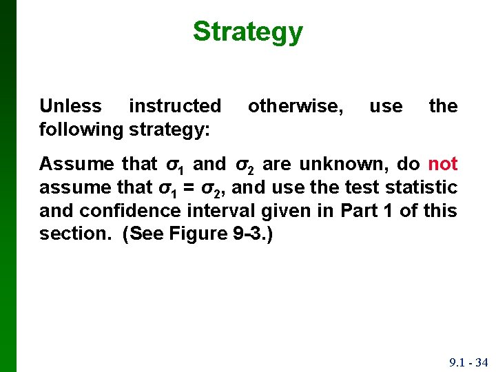
Strategy Unless instructed following strategy: otherwise, use the Assume that σ1 and σ2 are unknown, do not assume that σ1 = σ2, and use the test statistic and confidence interval given in Part 1 of this section. (See Figure 9 -3. ) 9. 1 - 34

9. 1 - 35

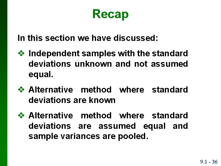
Recap In this section we have discussed: v Independent samples with the standard deviations unknown and not assumed equal. v Alternative method where standard deviations are known v Alternative method where standard deviations are assumed equal and sample variances are pooled. 9. 1 - 36