Inference issues in OLS Amine Ouazad Ass Prof

Inference issues in OLS Amine Ouazad Ass. Prof. of Economics

Outline 1. Heteroscedasticity 2. Clustering 3. Generalized Least Squares 1. For heteroscedasticity 2. For autocorrelation

HETEROSCEDASTICITY

Issue • The issue arises whenever the residual’s variance depends on the observation, or depends on the value of the covariates.

Example #1

Example #2 Here Var(y|x) is clearly increasing in x. Notice the underestimation of the size of the confidence intervals.

Visual checks with multiple variables • Use the vector of estimates b, and predict E(Y|X) using the predict xb, xb stata command. • Draw the scatter plot of the dependent y and the prediction Xb on the horizontal axis.

Causes • Unobservable that affects the variance of the residuals, but not the mean conditional on x. – y=a+bx+e. – with e=hz. The shock h satisfies E(h |x)=0, and E(z|x)=0 but the variance Var(z|x) depends on an unobservable z. – E(e|x)=0 (exogeneity), but Var(e|x)=Var(hz|x) depends on x. (previous example #1). • In practice, most regressions have heteroskedastic residuals.

Examples • Variability of stock returns depends on the industry. – Stock Returni, t = a + b Market Returnt + ei, t. • Variability of unemployment depends on the state/country. – Unemploymenti, t = a + b GDP Growtht + ei, t. • Notice that both the inclusion of industry/state dummies and controlling for heteroskedasticity may be necessary.

Heteroscedasticity: the framework • We set the ws so that their sum is equal to n, and they are all positive. The trace of the matrix W (see matrix appendix) is therefore equal to n.

Consequences 1. The OLS estimator is still unbiased, consistent and asymptotically normal (only depends on A 1 -A 3). 2. But the OLS estimator is then inefficient (the proof of the Gauss-Markov theorem relies on homoscedasticity). 3. And the confidence intervals calculated assuming homoscedasticity typically overestimate the power of the estimates/underestimate the size of the confidence intervals.

Variance-covariance matrix of the estimator • Asymptotically • At finite and fixed sample size • xi is the i-th vector of covariates, a vector of size K. • Notice that if the wi are all equal to 1, we are back to the homoscedastic case and we get Var(b|x) = s 2(X’X)-1 • We use the finite sample size formula to design an estimator of the variance-covariance matrix.

White Heteroscedasticity consistent estimator of the variance-covariance matrix • The formula uses the estimated residuals ei of each observation, using the OLS estimator of the coefficients. • This formula is consistent (plim Est. Asy. Var(b)=Var(b)), but may yield excessively large standard errors for small sample sizes. • This is the formula used by the Stata robust option. • From this, the square of the k-th diagonal element is the standard error of the k-th coefficient.

Test for heteroscedasticity • Null hypothesis H 0: si 2 = s 2 for all i=1, 2, …, n. • Alternative hypothesis Ha: at least one residual has a different variance. • Steps: 1. Estimate the OLS and predict the residuals ei. 2. Regress the square of the residuals on a constant, the covariates, their squares and their cross products (P covariates). 3. Under the null, all of the coefficients should be equal to 0, and NR 2 of the regression is distributed as a c 2 with P-1 degrees of freedom.

Suggests another visual check • Examples #1 and #2 with one covariate. • Example with two covariates.

Stata take aways • Always use robust standard errors – robust option available for most regressions. – This is regardless of the use of covariates. Adding a covariate does not free you from the burden of heteroscedasticity. • Test for heteroscedasticity: – hettest reports the chi-squared statistic with P-1 degrees of freedom, and the p-value. – A p-value lower than 0. 05 rejects the null at 95%. – The test may be used with small sample sizes, to avoid the use of robust standard errors.

CLUSTERING

Clustering, example #1 • Typical problem with clustering is the existence of a common unobservable component… – Common to all observations in a country, a state, a year, etc. • Take yit = xit + eit, a panel dataset where the residual eit=ui+hit. • Exercise: Calculate the variance-covariance matrix of the residuals.

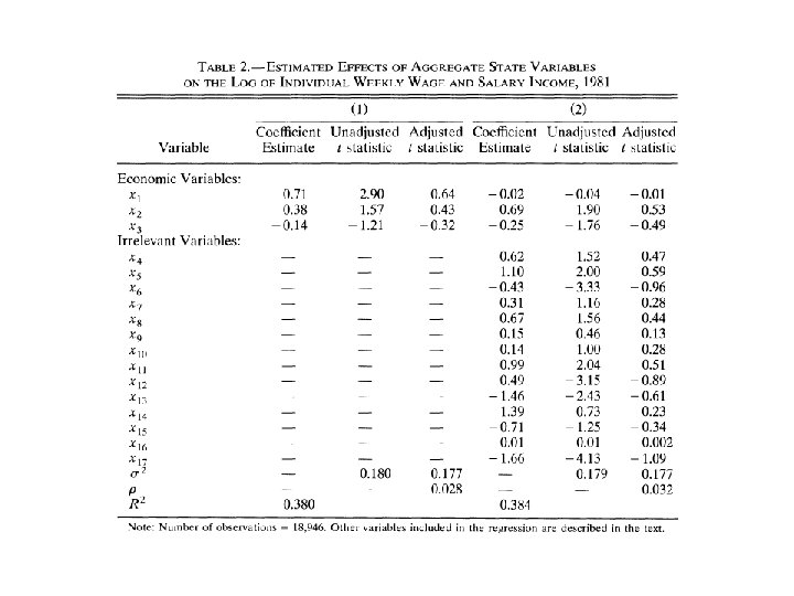
Clustering, example #2 • Other occurrence of clustering is the use of data at a higher level of aggregation than the individual observation. – Example: yij = xijb+zjg+eij. – This practically implies (but not theoretically), that Cov(eij, ei’j) is nonzero. • Example: – regression performanceit = c + d policyj(i) + eit. – regression stock returnit = constant + b Markett + eit.

Moulton paper

The clustering model • Notice that the variance-covariance matrix can be designed this way by blocks. • In this model, the estimator is unbiased and consistent, but inefficient and the estimated variance-covariance matrix is biased.

True variance-covariance matrix • With all the covariates fixed within group, the variance covariance matrix of the estimator is: • where m=n/p, the number of observations per group. • This formula is not exact when there are individual-specific covariates, but the term (1+(m-1)r) can be used as an approximate correction factor.

Descriptive Statistics

Stata • regress y x, cluster(unit) robust. – Clustering and robust s. e. s should be used at the same time. – This is the OLS estimator with corrected standard errors. – If x includes unit-specific variables, we cannot add a unit (state/firm/industry) dummy as well.

Multi-way clustering • Multi-way clustering: – “Robust inference with multi-way clustering”, Cameron, Gelbach and Miller, Technical NBER Working Paper Number 327 (2006). • Has become the new norm very recently. • Example: clustering by year and state. – yit = xitb + zig + wtd + eit – What do you expect? • ivreg 2 , cluster(id year). • ssc install ivreg 2.

GENERALIZED LEAST SQUARES

OLS is BLUE only under A 4 • OLS is not BLUE if the variance-covariance matrix of the residuals is not diagonal. • What should we do? • Take general OLS model Y=Xb+e. • And assume that Var(e)=W. • Then take the square root of the matrix, W-1/2. This is a matrix that satisfies W=(W-1/2 )’W-1/2. This matrix exists for any positive definite matrix.

Sphericized model • The sphericized model is: W-1/2 Y= W-1/2 Xb+ W-1/2 e • This model satisfies A 4 since Var(e|X)=s 2.

Generalized Least Squares • The GLS estimator is: • This estimator is BLUE. It is the efficient estimator of the parameter beta. • This estimator is also consistent and asymptotically normal. • Exercise: prove that the estimator is unbiased, and that the estimator is consistent.

Feasible Generalized Least Squares • The matrix W in general is unknown. We estimate W using a procedure (see later) so that plim W = W. • Then the FGLS estimator b=(X’W-1 X)-1 X’W-1 Y is a consistent estimator of b. • The typical problem is the estimation of W. There is no one size fits all estimation procedure.

GLS for heteroscedastic models • Taking the formula of the GLS estimator, with a diagonal variancecovariance matrix. • Where each weight is the inverse of wi. Or the inverse of si 2. Scaling the weights has no impact. • Stata application exercise: – Calculate weights and tse the weighted OLS estimator regress y x [aweight=w] to calculate the heteroscedastic GLS estimator, on a dataset of your choice.

GLS for autocorrelation • Autocorrelation is pervasive in finance. Assume that et=ret-1+ht, (we say that et is AR(1)) where ht is the innovation, uncorrelated with et-1. • The problem is the estimation of r. Then a natural estimator of r is the coefficient of the regression of et on et-1. • Exercise 1 (for adv. students): find the inverse of W. • Exercise 2 (for adv. students): find W for an AR(2) process. • Exercise 3 (for adv. students): what about MA(2) ? • Variation: Panel specific AR(1) structure.

Autocorrelation example

GLS for clustered models • Correlation r within each group. • Exercise: write down the variance-covariance matrix W of the residuals. • Put forward an estimator of r. • What is the GLS estimator of b in Y=Xb+e with clustering? • Estimation using xtgls, re.

Applications of GLS • The Generalized Least Squares model is seldom used. In practice, the variance of the OLS estimator is corrected for heteroscedasticity or clustering. – Take-away: use regress , cluster(. ) robust – Otherwise: xtgls, panels(hetero) – xtgls, panels(correlated) – xtgls, panels(hetero) corr(ar 1) • The GLS is mostly used for the estimation of random effects models. – xtreg, re

CONCLUSION: NO WORRIES

Take away for this session 1. Use regress, robust; always, unless the sample size is small. 2. Use regress, robust cluster(unit) if: – You believe there are common shocks at the unit level. – You have included unit level covariates. 3. Use ivreg 2, cluster(unit 1 unit 2) for two way clustering. 4. Use xtgls for the efficient FGLS estimator with correlated, AR(1) or heteroscedastic residuals. – This might allow you to shrink the confidence intervals further, but beware that this is less standard than the previous methods.