Simultaneity Issues in Ordinary Least Squares Amine Ouazad

Simultaneity Issues in Ordinary Least Squares Amine Ouazad Ass. Prof. of Economics

Recap from last sessions • OLS is consistent under the linearity assumptions, the full rank assumption, and the exogeneity of the covariates assumption. • The exogeneity of the covariates (A 3) is violated whenever: 1. 2. 3. • • • There is an omitted variable in the residual which is correlated with the covariates. (last session) There is measurement error. (last session) There is a reverse causality or simultaneity problem (this session). These three issues cause identification problems: even if sample size is infinite, the estimator does not come arbitrarily close to the true value. The OLS estimator is inconsistent. The OLS estimator is biased.

Outline 1. Supply/demand estimation 2. Simultaneous Equation Model (X Rated) 3. Bruce Sacerdote, Peer effects with random assignment: Results for Dartmouth roommates, Quarterly Journal of Economics, 2001.

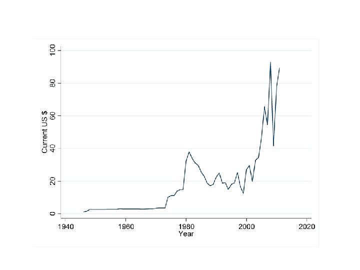
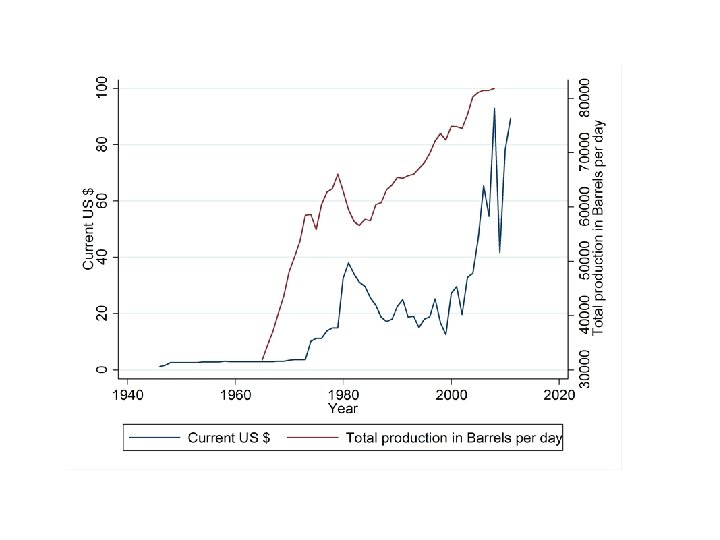
SUPPLY AND DEMAND ESTIMATION

Source: BP Statistical Review, 2009. Forecastchart. com

Supply/demand estimation The problem • pt : price at time t. • qt : quantity at time t. • Specification: qt = a + b pt + e. • The OLS regression of qt on pt does not satisfy A 3 because there is a correlation between price changes and the unobservables e.

Full model • qt, pt: endogenous variables. • e: supply shock, u: demand shock. Market equilibrium: Notice the effect of supply and demand shocks on price and quantity. Hence Cov(pt, et) is non zero and the regression of quantity on prices does not yield a consistent estimator of either demand or supply.

Exogenous/Endogenous • Greek: ενδογενής, meaning "proceeding from within" ("ενδο"=inside "-γενής"=coming from), the complement of exogenous (Greek: εξωγενής exo, "έξω"= outside) "proceeding from outside". • Definition of exogenous/endogenous depends on the model. For instance, in the previous model, if

Structural, Identifiable Parameters • Structural parameters: (a, b, c, d, Var(e), Var(u)) • Identifiable parameters: – These parameters are the mean of pt, the mean of qt, the variance of pt, the variance of qt. • Hence there are 4 identifiable parameters, and 6 structural parameters…. The model is not identified.

Observational equivalence, example • With Cov(et, ut) = 0, Var(et) = 1, Var(ut) =1. • Then, the following demand supply schedule gives the same distributions of prices, quantities, and correlation between price and quantity: • How did I find this? ?

Solving the simultaneity problem

Intuition • If you have a variable that affects demand without affecting supply, then it is possible to identify the supply curve. • If you have a variable that affects supply without affecting demand, then it is possible to identify the demand curve. • Here we have this: – temperature affects only supply ! – We are able to estimate the demand curve. How ?

Consider the following: • Prove that this covariance is equal to b. – Under what assumption? • z is called a supply shifter. – A supply shifter identifies demand. • Question: what if you had one variable that affects demand without affecting supply?

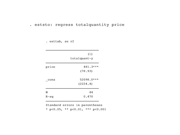
Stata application ivreg quantity (price = temperature) • This regression estimates the demand curve, since temperature affects only supply. • This is called an instrumental variable regression, to be seen later in econometrics A.

(Reference: William Greene, Simultaneous Equations Model) SIMULTANEOUS EQUATIONS

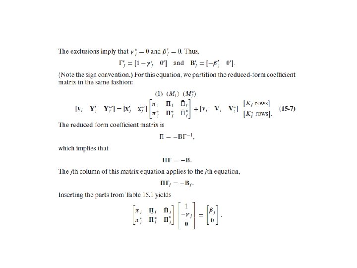
Structural form of the model • • yt 1, yt. M are the endogenous variables xt 1, xt. K are the exogenous variables. et 1, …, et. M are the structural residuals/shocks/unobservables. t: time periods. In matrix form:

Reduced form of the model •

Exercise • Write the structural form of the model for the oil example. • Hints: – There are 2 equations. – 2 Endogenous variables: pt qt. – 1 Exogenous variable: the constant. • Write the reduced form model using the previous formula. Do we find the same solution?

Matrix form notation: Structural model • Y : Tx. M matrix. T rows, M columns. – M = 2 in the oil example. • X: Tx. K matrix. – K = 1 in the oil example. • E : Tx. M vector. • Exogeneity E(E|X) = 0 and E(E’E|X) = S.

Matrix form notation: Reduced form model • P : the matrix of reduced form parameters. (Kx. M matrix). • V : the vector of residuals, with variancecovariance matrix W. The var-cov matrix has size M.

Identification of Reduced Form parameters • Parameters in the structural form model: – M*M + K*M + ½ M(M+1) – G matrix, B matrix, S matrix. • Parameters in the reduced form model: – K*M + ½ M(M+1) – P matrix, W matrix. • Aie ! M*M parameters ‘too many’ !

Solutions? 1. Normalizations: – make the coefficient of each independent variable equal to 1. The number of excess parameters is then M(M-1). 2. Identities & Restrictions: – Pin down relationships between parameters. 3. Exclusions: – Political events have an effect on supply, but not on world demand. 4. Restrictions on the variance covariance matrix: – Assume 0 correlation between disturbances in the reduced form model.

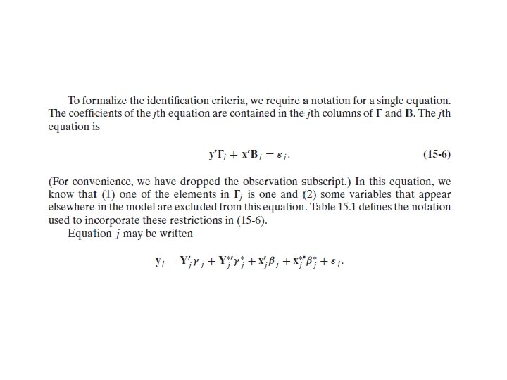
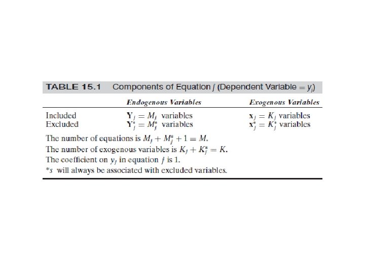
Notations for equation j • Considering equation j in isolation… • We set the coefficient on yj equal to 1. • We are going to exclude endogenous variables (exactly Mj* variables) and exclude exogenous variables (Kj* variables).

Equation j

Finding the structural parameters Pj*gj=pj* • This equation gives the structural parameters of equation j. It has Kj* equations (the rows of Pj*) and Mj unknowns (the coefficients of the structural parameters).

Order condition Kj* greater or equal than Mj • The number of exogenous variables excluded in equation j must be at least as large as the number of endogenous variables included in equation j. • Relationship with agricultural product exercise? ?

Rank condition rank[Pj*] = Mj • This condition imposes a restriction on the submatrix of the reduced-form coefficient matrix.

Deducing the coefficients of the exogenous variables • This equation gives the coefficients of the exogenous covariates of equation j as a function of known quantities.

Take Away • With simultaneous equations, only the reduced-form model is typically identified in OLS. – You cannot interpret the results of an OLS of the structural model (where endogenous variables are in the covariates). • However, by making suitable assumptions on the exclusion of exogenous variables, you can identify the model.

Take Away • 4 steps: 1. Estimate the reduced form model. 2. Make the necessary exclusion restrictions. 3. Write the structural parameters as a function of the reduced form parameters. 4. Solve the system of equations.

SOCIAL INTERACTIONS: SACERDOTE QJE 2001

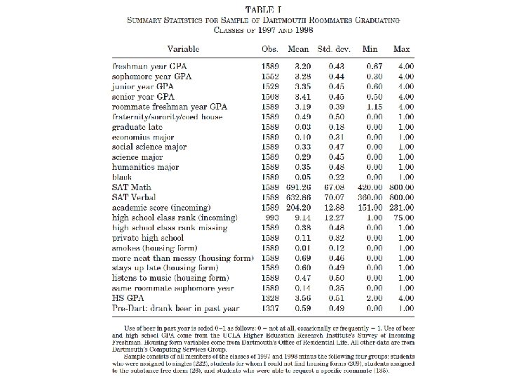
The question • What is the impact of a roommate’s characteristic and behavior on your GPA/behavior ? – Characteristic: SAT score (before university), gender, age, any x that is not changing over time. – Behavior: any variable that is a choice, such as choice of major, achievement.

The issues • Regressing my GPA on the GPA of my roommate has a number of problems… – First, the GPA of my roommate is also determined by my GPA: simultaneity bias. (A 3) – Second, if roommates are not randomly allocated, and if, for instance, having a male roommate is correlated with having a drinking roommate, then: omitted variable bias. (A 3) – Third, there are some common shocks that affect both me and my roommate at the same time: correlation of the error terms. (A 4) – Fourth, the effect of my roommate may depend on my characteristics, and also on his other characteristics: non linearity. (A 1)

The structural model • Academic ability, Measurement error, Grade point average of the roommate, residual. • Assumptions A 1, A 2 are maintained. The exogeneity of the GPA of the other roommate (A 3) is violated.

The reduced form model • Notice that right-hand side variables are purely exogenous. • Identification problem is given pi_0, pi_1, and pi_2, can we “get” the structural parameters? Without any more constraint, no. • Notice that there will be correlation of the residuals across individuals.

Identification problem • In the reduced form, assuming A 1, A 2, A 3, the OLS is consistent. A 4 is violated (more on this in the next session). – regress gpa_roommate characteristics_roommate gives consistent and unbiased estimates of the effects. • (To correct for A 4, add option cluster(room) if room is a variable indicating the room number).

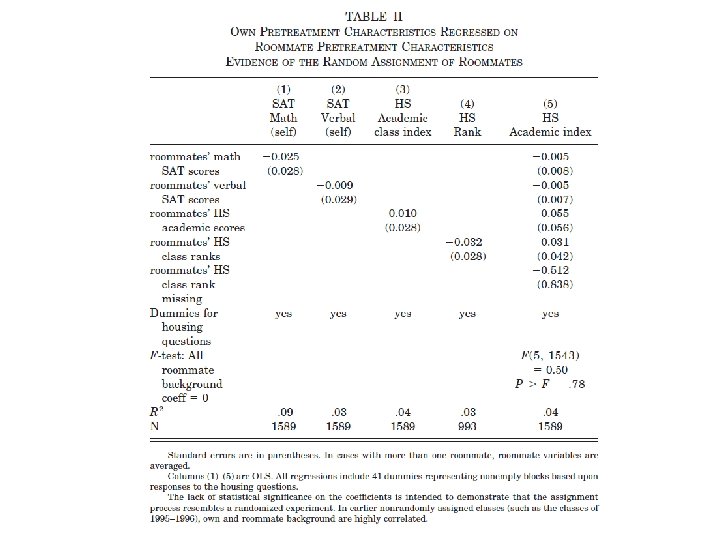
Randomization • Individuals are randomized conditionally on their stated preferences. Violation of A 3? Not if the preferences are present as covariates. – Conditional randomization, E(e|X) = 0. • Method of randomization?

Results

Checking Linearity (A 1)

Take Away from this session • Spot Reverse Causality issues in papers! – Sometimes mild, sometimes very severe (demand/supply, social interactions) • You can solve the problem by instrumenting the endogenous variable with a variable that affects the variable without affecting the outcome (a demand shifter for supply, a supply shifter for demand).

OLS: Three identification issues 1. Measurement error 2. Omitted variable bias 3. Reverse causality/Simultaneity