Imagen de resonancia magntica http www cis rit

Imagen de resonancia magnética http: //www. cis. rit. edu/htbooks/mri/inside. htm Magnetic resonance imaging, G. A. WRIGHT IEEE SIGNAL PROCESSING MAGAZINE pp: 56 -66 JANUARY 1997

MRI Timeline 1946 MR phenomenon - Bloch & Purcell 1952 Nobel Prize - Bloch & Purcell 1950 NMR developed as analytical tool 1960 1972 Computerized Tomography 1973 Backprojection MRI - Lauterbur 1975 Fourier Imaging - Ernst 1977 Echo-planar imaging - Mansfield 1980 FT MRI demonstrated - Edelstein 1986 Gradient Echo Imaging NMR Microscope 1987 MR Angiography - Dumoulin 1991 Nobel Prize - Ernst 1992 Functional MRI 1994 Hyperpolarized 129 Xe Imaging 2003 Nobel Prize - Lauterbur & Mansfield

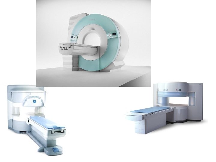
Modelos de scanners

Algunas bobinas de GE

Doty coils

Tomographic imaging Magnetic resonance started out as a tomographic imaging modality for producing NMR images of a slice through the human body.

Magnetic resonance imaging is based on the absorption and emission of energy in the radio frequency range of the electromagnetic spectrum. Many scientists were taught that you can not image objects smaller than the wavelength of the energy being used to image. MRI gets around this limitation by producing images based on spatial variations in the phase and frequency of the radio frequency energy being absorbed and emitted by the imaged object.

Microscopic Property Responsible for MRI The human body is primarily fat and water. Fat and water have many hydrogen atoms which make the human body approximately 63% hydrogen atoms. Hydrogen nuclei have an NMR signal. For these reasons magnetic resonance imaging primarily images the NMR signal from the hydrogen nuclei. The proton possesses a property called spin which: 1. can be thought of as a small magnetic field, and 2. will cause the nucleus to produce an NMR signal.

Basic physics Magnetic resonance imaging, G. A. WRIGHT IEEE SIGNAL PROCESSING MAGAZINE pp: 56 -66 JANUARY 1997

The relevant property of the proton is its spin, I, and a simple classical picture of spin is a charge distribution in the nucleus rotating around an axis collinear with I. The resulting current has an associated dipole magnetic moment, p, collinear with I, and the quantum mechanical relationship between the two is where h is Planck’s constant and y is the gyromagnetic ratio. For protons, y/2 n = 42. 6 MHz/T.

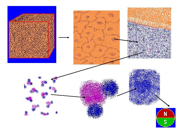
In a single-volume element corresponding to a pixel in an MR image, there are many protons, each with an associated dipole magnetic moment, and the net magnetization, M = Mx j+ Myi + Mzk, of the volume element is the vector sum of the individual dipole moments, where i, j, and k are unit vectors along the x, y , and z axes, respectively. In the absence of a magnetic field, the spatial orientation of each dipole moment is random and M = 0.

This situation is changed by a static magnetic field, Bo =Bok. This field induces magnetic moments to align themselves in its direction, partially overcoming thermal randomization so that, in equilibrium, the net magnetization, M =M 0 k, represents a small fraction (determined from the Boltzmann distribution) of times the total number of protons. While the fraction is small, the total number of contributing protons is very large at approximately 10'' dipoles in a S mm 3 volume.

Equilibrium is not achieved instantaneously. Rather, from the time the static field is turned on, M grows from zero toward its equilibrium value M, along the z axis; that is, where T 1 is the longitudinal relaxation time. This equation expresses the dynamical behavior of the component of the net magnetization Mz along the longitudinal (z) axis.

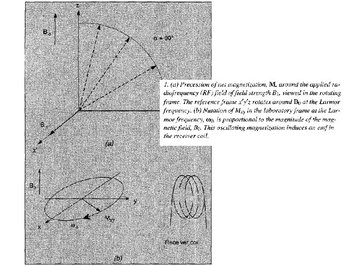
The component of the net magnetization, Mxy, which lies in the transverse plane orthogonal to the longitudinal axis, undergoes completely different dynamics. Mxy, often referred to as the transverse magnetization, can be described by acomplex quantity where This componentprecesses about Bo, i. e. , The precession frequency is proportional to B, and is referred to as the Larmor frequency (Fig. 1 b). This relation holds at the level of individual dipoles as well, so that

Accompanying any rotating dipole magnetic moment is a radiated electromagnetic signal circularly polarized about the axis of precession; this is the signal detected in MRI. The usual receiver is a coil, resonant at w 0 , whose axis lies in the transverse plane-as Mxy, precesses, it induces an electromotive force (emf) in the coil.

If Bo induces a collinear equilibrium magnetization M, how can we produce precessing magnetization orthogonal to Bo? The answer is to apply a second, time-varying magnetic field that lies in the plane transverse to Bo This field rotates about the static field direction k at radian frequency w 0 If we then place ourselves in a frame of reference (x'y'z) that also rotates at radian frequency w 0, this second field appears stationary.

Moreover, any magnetization component orthogonal to B 0, no longer appears to rotate about Bo. Instead, in this rotating frame, M appears to precess about the "stationary" field B 1, alone with radian frequency. One can therefore choose the duration of B 1, so that M is rotated into the transverse plane. The corresponding B 1 waveform is called a 90" excitation pulse

The signal from Mxy will eventually decay. • Part of this decay is the result of the drive to thermal equilibrium where M is brought parallel to Bo, as described earlier. • Over time, the vector sum, M, decreases in magnitude since the individual dipole moments no longer add constructively. The associated decay is characterized by an exponential with time constant T 2*

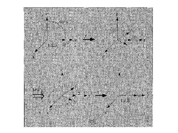
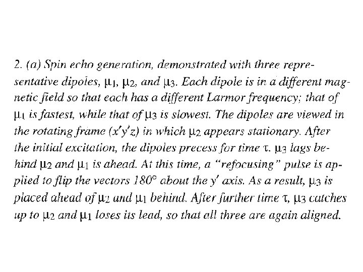
the loss of transverse magnetization due to dephasing can be recovered to some extent by inducing a spin echo. Specifically, let the dipole moments evolve for a time t after excitation. At this time apply another B 1 field along y' to rotate the dipole moments 180" around B 1. This occurs in a time that is very short compared to t. This pulse effectively negates the phase of the individual dipole moments that have developed relative to the axis of rotation of the refocusing pulse. Assuming the precession frequencies of the individual dipole moments remain unchanged then at a time , t, after the spin-echo or 180" pulse, the original contributions of the individual dipoles refocus (Fig. 2 a). Hence, at a time TE = 2 t after the excitation, the net magnetization is the same as it was just after excitation.

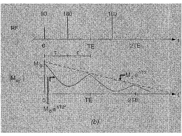
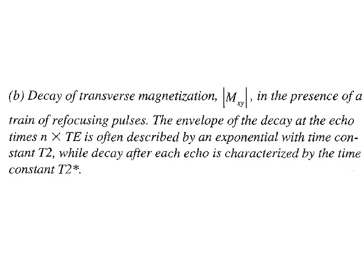
If one applies a periodically spaced train of such 180" pulses following a single excitation, one observes that the envelope defined by at each echo time steadily decays (Fig. 2 b). This irreversible signal loss is often modeled by an exponential decay with time constant T 2. the transverse relaxation time:

Before the experiment can he repeated with another excitation pulse, sufficient time must elapse to re-establish equilibrium magnetization along k. As indicated in Eq. (l), a sequence repetition time, TR, of several Tls is necessary for full recovery of equilibrium magnetization, Mo, along Mz, between excitations. Bloch equation

Imaging, contrast and noise

Imaging: spatial resoltion of the signal Two-step process: (i) exciting the magnetization into the transverse plane over a spatially restricted region, and (ii) encoding spatial location of the signal during data acquisition.

Spatially Selective Excitation The usual goal in spatially selective excitation is to tip magnetization in a thin spatial slice or section along the z axis, into the transverse plane. Conceptually, this is accomplished by first causing the Larmor frequency to vary linearly in one spatial dimension, and then, while holding the field constant, applying a radiofrequency (RF) excitation pulse crafted to contain significant energy only over a limited range of temporal frequencies (BW) corresponding to the Larmor frequencies in the slice.

To a first approximation, the amplitude of the component at each frequency in the excitation signal determines the flip angle of the protons resonating at that frequency. If the temporal Fourier transform of the pulse has a rectangular distribution about w 0, a rectangular distribution of spins around zo is tipped away from the z axis over a spatial extent

For small tip angles we can solve the Bloch equations explicitly to get the spatial distribution of Mxy following an RF pulse, B 1(t), in the presence of a magnetic field gradient of amplitude Gz: Assume that all the magnetization initially lies along the z axis. Under these conditions, a rectangular slice profile is achieved if

Image Formation Through S p a t i a l Frequency Encoding The Imaging Equation Once one has isolated a volume of interest using selective excitation, the volume can be imaged by manipulating the precession frequency (determined by the Larmor relation), and hence the phase of Mxy. For example, introduce a linear magnetic field gradient, Gx, in the x direction so that each dipole now contributes a signal at a frequency proportional to its x-axis coordinate.

In principle, by performing a Fourier transform on the received signal, one can determine Mxy as a function of x. An equivalent point of view follows from observing that each dipole contributes a signal with a phase that depends linearly on its x-axis coordinate and time. Thus, the signal as a whole samples the spatial Fourier transform of the image along the kx spatial frequency axis, with the sampled location moving along this axis linearly with time.

A more general viewpoint can be developed mathematically from the Bloch equation. Using spatially selective excitation only protons in a thin slice at z = zo are tipped into the transverse plane so that Let the magnetic field after excitation be

Assume is relatively constant during data acquisition (i. e. acquisition duration << Tl, T 2*); and let the time at the center of the acquisition be tacq. During acquisition

The signal received, S(t), is the integral of this signal over the xy plane.

If this signal is demodulated by w 0 then the resulting baseband signal, Se(kx(t), ky(t)), is the 2 D spatial Fourier transform of at spatial frequency coordinates kx(t) and ky(t). One chooses Gx(t) and Gy(t) so that, over the full data acquisition, the 2 D frequency domain is adequately sampled and the desired image can be reconstructed as the inverse Fourier transform of the acquired data.