Image Space Rendering and Texturing Celine Loscos 2004

Image Space Rendering and Texturing ©Celine Loscos 2004 Anthony Steed 1999

Introduction • We are interested in the process of displaying the scene in the drawing window • In other words, we are interested in choosing a colour for each pixel depending on how each polygon is viewed from the viewpoint

Introduction • One way is with ray tracing: – trace a ray from each pixel, and intersect it with the polygons of the scene – Problem: This is expensive • We are looking for methods that project the polygons on the window, and then decisions on the pixel colour are made in the image space

Overview • • Coping with depth Gouraud shading Phong shading Texturing

Coping with depth • When all polygons are projected on the screen, they may overlap • The problem is to know which one is in front of the others • There are several methods to treat this – – Scan-line depth buffering Z-buffer Recursive sub-division Trade-offs • Z stands for the depth

Scan-line depth buffering: Extending the AET (active edge table) • Easy enough if polygon do NOT intersect • Put all polygon edges into ET with extra depth information and proceed as before except … • … now consider overlapping ranges of edges

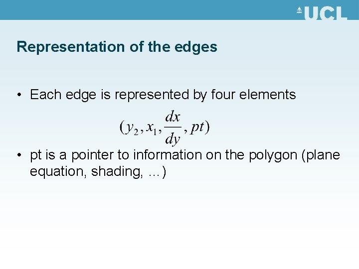
Representation of the edges • Each edge is represented by four elements • pt is a pointer to information on the polygon (plane equation, shading, …)

AET Example

AET Example Notes • Our edge table must contain data which enables us to look up z at at intersection point • From x 1 to x 2 only A is considered. • At x 2 A and B are considered – plane equations are solved to get depth at (x 2, i) – A is closest so x 2 to x 3 is filled as A • At x 3 A finishes so we draw B from x 3 to x 4 • At x 4 B and C are considered, B in front etc…

Method analysis • Drawbacks – Sorting is required into the AET – If the number of polygons is high, the z-computation will be costly • Accelerations • Would usually store the scanning in a 1 D BSP tree for large numbers of polygons! • Exploit coherence (assume similar overlapping at y+1) • Pre-order the polygons (no need to compute the depth calculations)

Zbuffer • Don’t bother with per span tests - just test every pixel • Most common usage is a full window sized array ZBUF (M*N) of 16, 24 or 32 bit “depth” values • Basic idea: – Initialise Zbuffer to Z_MAX – For each polygon • Point (x, y, z) of the polygon projects on pixel (xs, ys) and has colour col associated • If z < ZBUF[x, y] set CBUF[x, y] = col else do nothing

Use of the polygon scan-line renderer • We can do this in several ways • 1 D z-buffer re-used on each scan line – Process each polygon with separate AET – Or use as adjunct to extended AET for multiple polygons • Problems … – Aliasing on depth (z-buffer tearing)

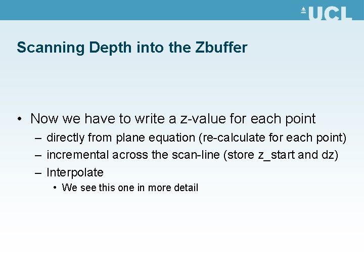
Scanning Depth into the Zbuffer • Now we have to write a z-value for each point – directly from plane equation (re-calculate for each point) – incremental across the scan-line (store z_start and dz) – Interpolate • We see this one in more detail

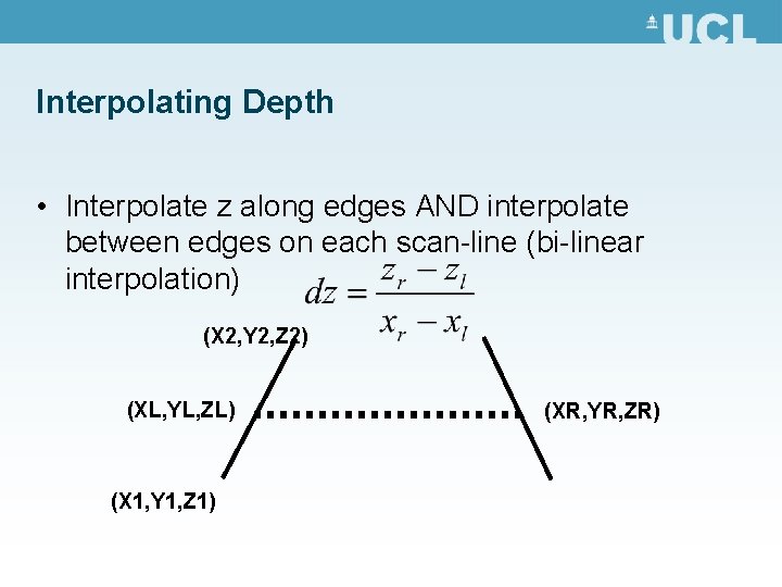
Interpolating Depth • Interpolate z along edges AND interpolate between edges on each scan-line (bi-linear interpolation) (X 2, Y 2, Z 2) (XL, YL, ZL) (X 1, Y 1, Z 1) (XR, YR, ZR)

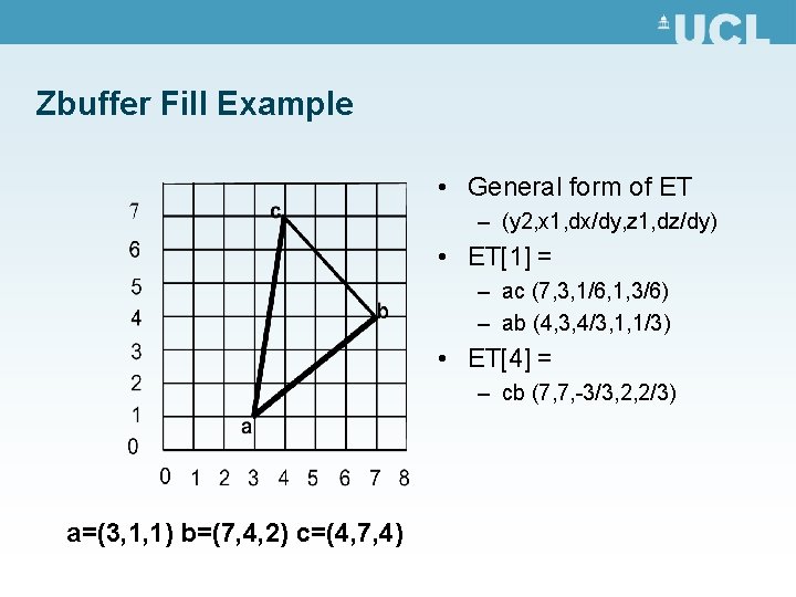
Zbuffer Fill Example • General form of ET – (y 2, x 1, dx/dy, z 1, dz/dy) • ET[1] = – ac (7, 3, 1/6, 1, 3/6) – ab (4, 3, 4/3, 1, 1/3) • ET[4] = – cb (7, 7, -3/3, 2, 2/3) a=(3, 1, 1) b=(7, 4, 2) c=(4, 7, 4)

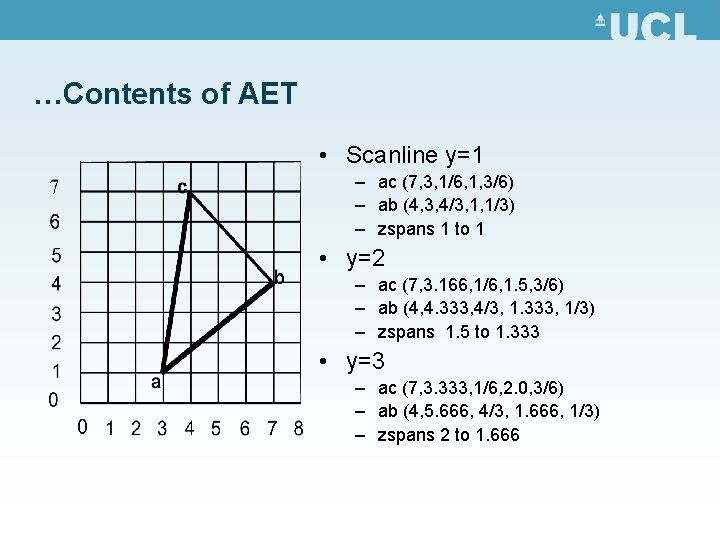
…Contents of AET • Scanline y=1 – ac (7, 3, 1/6, 1, 3/6) – ab (4, 3, 4/3, 1, 1/3) – zspans 1 to 1 • y=2 – ac (7, 3. 166, 1/6, 1. 5, 3/6) – ab (4, 4. 333, 4/3, 1. 333, 1/3) – zspans 1. 5 to 1. 333 • y=3 – ac (7, 3. 333, 1/6, 2. 0, 3/6) – ab (4, 5. 666, 4/3, 1. 666, 1/3) – zspans 2 to 1. 666

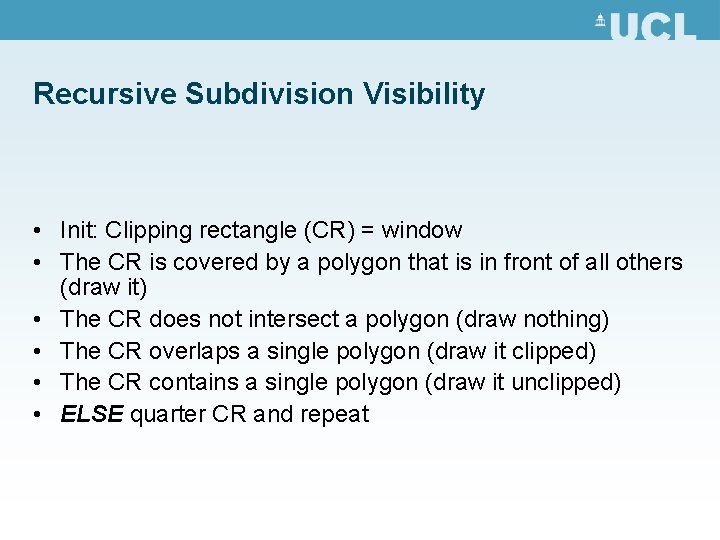
Recursive Subdivision Visibility • Init: Clipping rectangle (CR) = window • The CR is covered by a polygon that is in front of all others (draw it) • The CR does not intersect a polygon (draw nothing) • The CR overlaps a single polygon (draw it clipped) • The CR contains a single polygon (draw it unclipped) • ELSE quarter CR and repeat

Trade-Offs • Zbuffer can be inaccurate with few bits – really simple to implement though! • Scan-line AET good for large polygons – good coherency across lines – requires non-intersecting polygons • zbuffer good for small, sparse polygons – AET more time consuming to maintain

Choosing the colour • Gouraud shading • Phong shading • Texture mapping

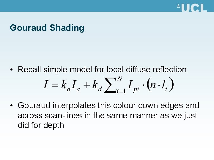
Gouraud Shading • Recall simple model for local diffuse reflection • Gouraud interpolates this colour down edges and across scan-lines in the same manner as we just did for depth

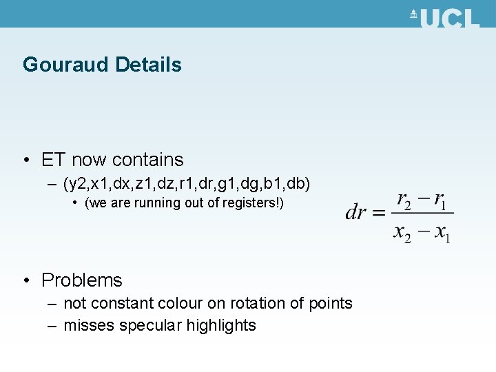
Gouraud Details • ET now contains – (y 2, x 1, dx, z 1, dz, r 1, dr, g 1, dg, b 1, db) • (we are running out of registers!) • Problems – not constant colour on rotation of points – misses specular highlights

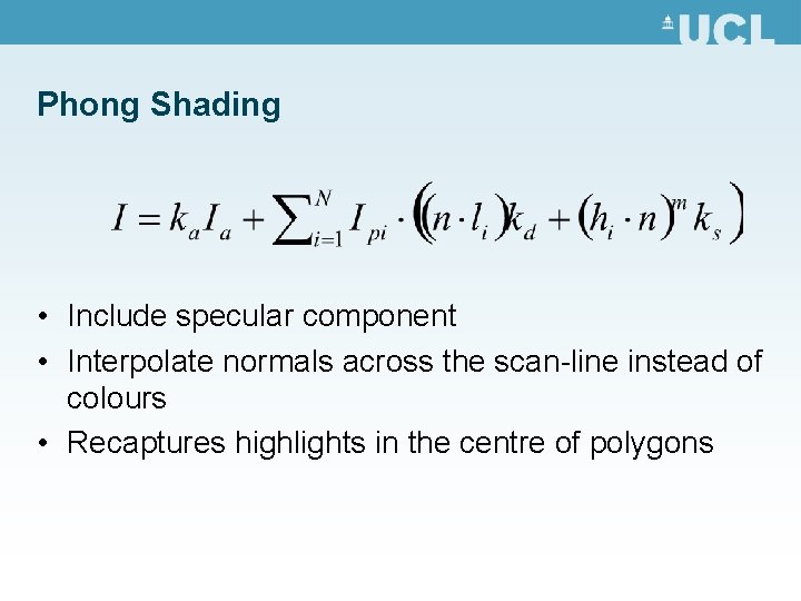
Phong Shading • Include specular component • Interpolate normals across the scan-line instead of colours • Recaptures highlights in the centre of polygons

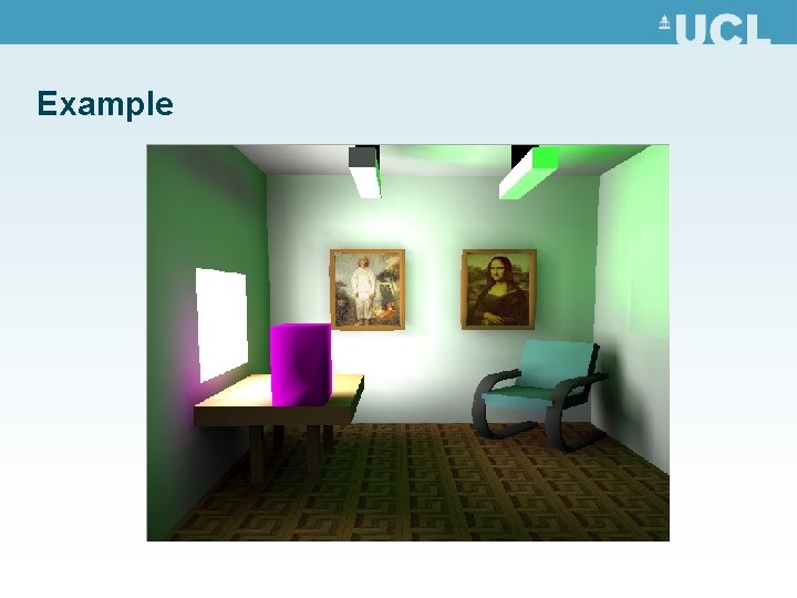
Texture mapping • We have seen that a colour can be assigned to a polygon, or to each vertex • Now if we consider small details, we may not want to add polygons to represent every detail • We prefer to keep a large polygon and use an image to represent the details

Example

Texture Mapping • Why? – Approximation for surface colouring – Efficient packing of flat detail • Standard texture mapping modifies diffuse mapping – Pasting a picture onto the polygon • A texture is a 2 D array of texels storing RGB or RGBA components

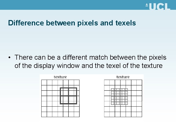
Difference between pixels and texels • There can be a different match between the pixels of the display window and the texel of the texture

Overview • Texture mapping – Inverse and Forward Mapping – Bilinear interpolation – Perspective correction • Mipmapping • Other forms of mapping – Environment – Bump mapping

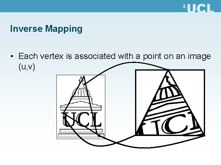
Inverse Mapping • Each vertex is associated with a point on an image (u, v)

Forward Mapping • For points in the image, map onto the polygon – much harder to implement correctly, and harder to model • Inverse mapping is much more commonly used – Most 3 D modelers output U, V co-ordinates for texture application

Quick and Dirty Solution • Yet more parameters in the ET! • Bilinear interpolation of u&v down polygon edges, and across scan-lines • Works, but is very ugly – Does not consider fore-shortening of image in depth

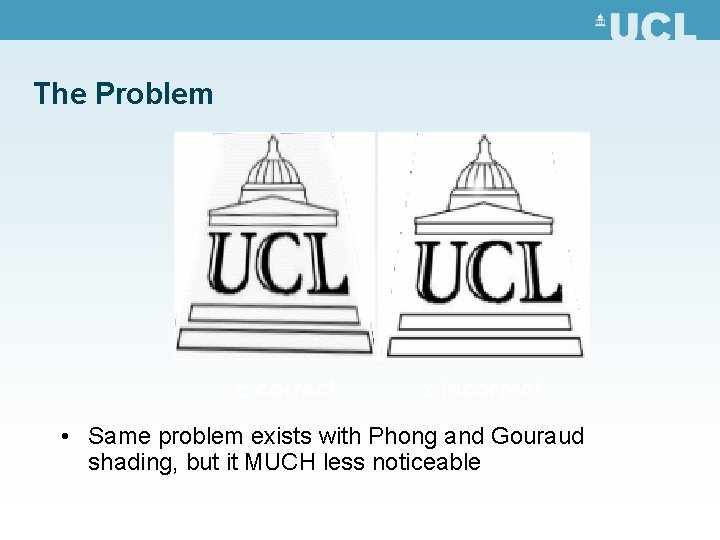
The Problem z correct z incorrect • Same problem exists with Phong and Gouraud shading, but it MUCH less noticeable

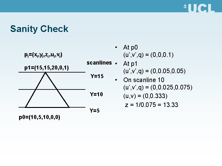
The Solution • Need to compensate fore-shortening by interpolating over 1/z • Interpolate (u’, v’, q) where q=1/z – At vertices we know (u 1, v 1, z 1), (u 2, v 2, z 2) – Interpolate between (u 1 / z 1, v 1 / z 1, 1/z 1) and (u 2/z 2, v 2 / z 2, 1/z 2) to get (u’, v’, q) – Restore u, v, by dividing u’ and v’ by q

Sanity Check pi=(xi, yi, zi, ui, vi) p 1=(15, 20, 0, 1) • At p 0 (u’, v’, q) = (0, 0, 0. 1) scanlines • At p 1 (u’, v’, q) = (0, 0. 05) Y=15 • On scanline 10 (u’, v’, q) = (0, 0. 025, 0. 075) Y=10 (u, v) = (0, 0. 333) z = 1/0. 075 = 13. 33 Y=5 p 0=(10, 5, 10, 0, 0)

Minor Issues • Now have two divisions per pixel! • Some optimisations – only do the division at end of the spans and interpolate across spans – or only do the division every n pixels • Remaining problem – we have not touched upon how to clip u, v values in 3 D or 2 D!

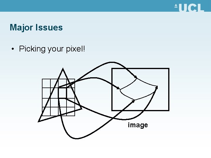
Major Issues • Picking your pixel! image

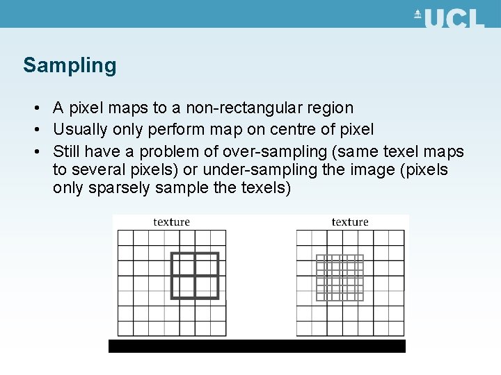
Sampling • A pixel maps to a non-rectangular region • Usually only perform map on centre of pixel • Still have a problem of over-sampling (same texel maps to several pixels) or under-sampling the image (pixels only sparsely sample the texels)

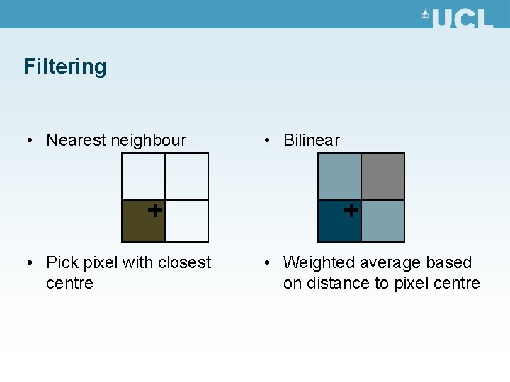
Filtering • Nearest neighbour • Bilinear • Pick pixel with closest centre • Weighted average based on distance to pixel centre

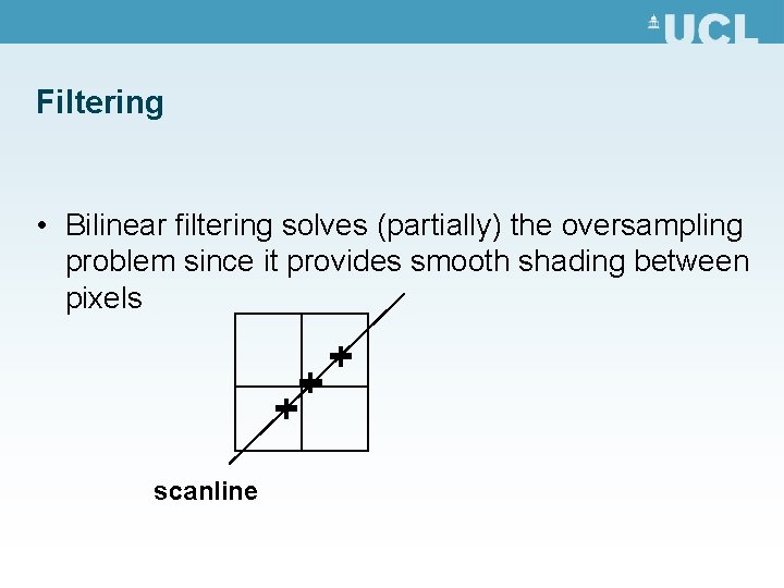
Filtering • Bilinear filtering solves (partially) the oversampling problem since it provides smooth shading between pixels scanline

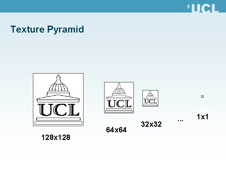
Mip-Mapping • • When undersampling we use mippmapping Resample image at lower resolution Create a “pyramid” of textures. Interpolate texture between two adjacent layers

Texture Pyramid 128 x 128 64 x 64 32 x 32 . . . 1 x 1

Sampling • Choose two layers based on texel span – Choice is made selecting the two levels where the dv and dv for dx and dy are closest to one • Interpolate between four pixels in higher layer and one in lower layer

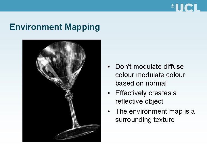
Environment Mapping • Don’t modulate diffuse colour modulate colour based on normal • Effectively creates a reflective object • The environment map is a surrounding texture

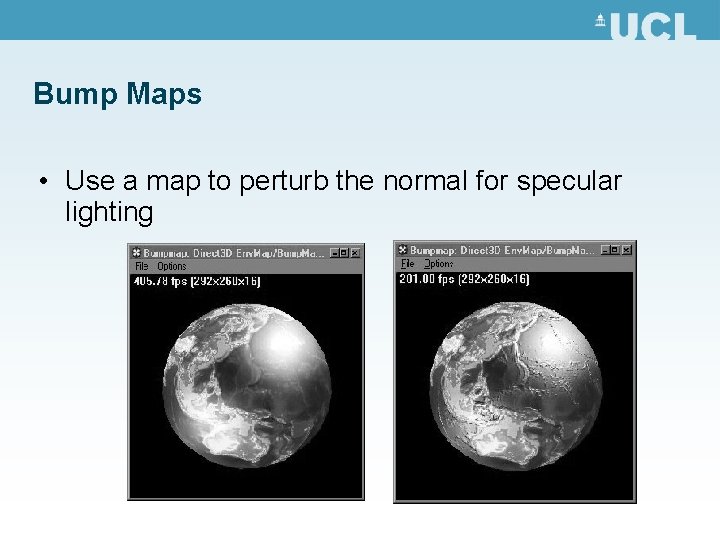
Bump Maps • Use a map to perturb the normal for specular lighting