High Performance Computing of Fast Independent Component Analysis

High Performance Computing of Fast Independent Component Analysis for Hyperspectral Image Dimensionality Reduction on MIC-based Clusters Minquan Fang, Yi Yu, Weimin Zhang, Heng Wu, Mingzhu Deng, Jianbin Fang （National University of Defence Technology）

Outline • 1. Motivation • 2. Fast. ICA and its Hotspots • 3. Parallelization and Optimization – – – Covariance matrix calculation White processing ICA iteration • 4. Ms-Fast. ICA and Experimental Result • 5. Conclusions

Outline • 1. Motivation • 2. Fast. ICA and its Hotspots • 3. Parallelization and Optimization – – – Covariance matrix calculation White processing ICA iteration • 4. Ms-Fast. ICA and Experimental Result • 5. Conclusions

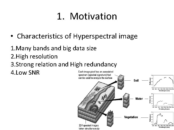
1. Motivation • Characteristics of Hyperspectral image 1. Many bands and big data size 2. High resolution 3. Strong relation and High redundancy 4. Low SNR

1. Motivation • Necessity for dimensionality reduction – 1. curse of dimensionality – 2. hardly train for sample categories – 3. empty space phenomenon

1. Motivation • Complexity for dimensionality reduction – Matrix calculation, iterations and large-scale loops • Requirement for dimensionality reduction – real time Time is consuming and parallel computing is needed

1. Motivation • hyperspectral image dimensionality reduction methods – PCA(principal component analysis) – ICA(independent component analysis) • Fast. ICA is a variant of ICA that converges fast – ISOMAP(isometric mapping) – LLE(local linear embedding) In this paper, we investigate Fast. ICA on MIC-based clusters

Outline • 1. Motivation • 2. Fast. ICA and its Hotspots • 3. Parallelization and Optimization – – – Covariance matrix calculation White processing ICA iteration • 4. Ms-Fast. ICA and Experimental Result • 5. Conclusions

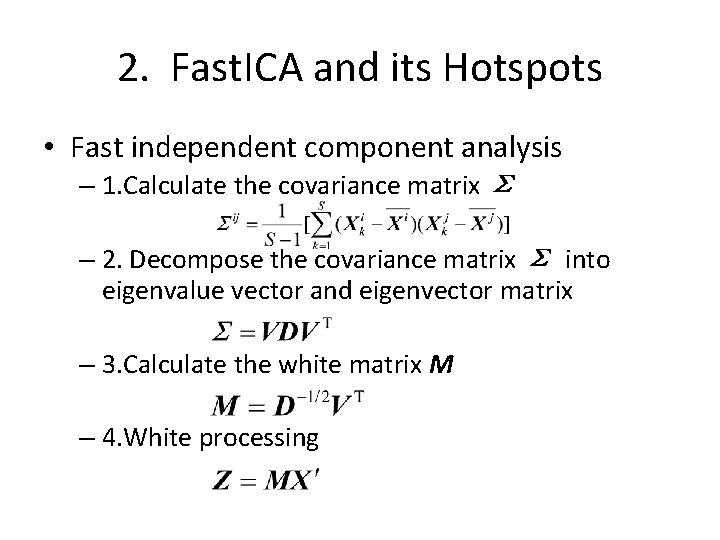
2. Fast. ICA and its Hotspots • Fast independent component analysis – 1. Calculate the covariance matrix Σ – 2. Decompose the covariance matrix Σ into eigenvalue vector and eigenvector matrix – 3. Calculate the white matrix M – 4. White processing

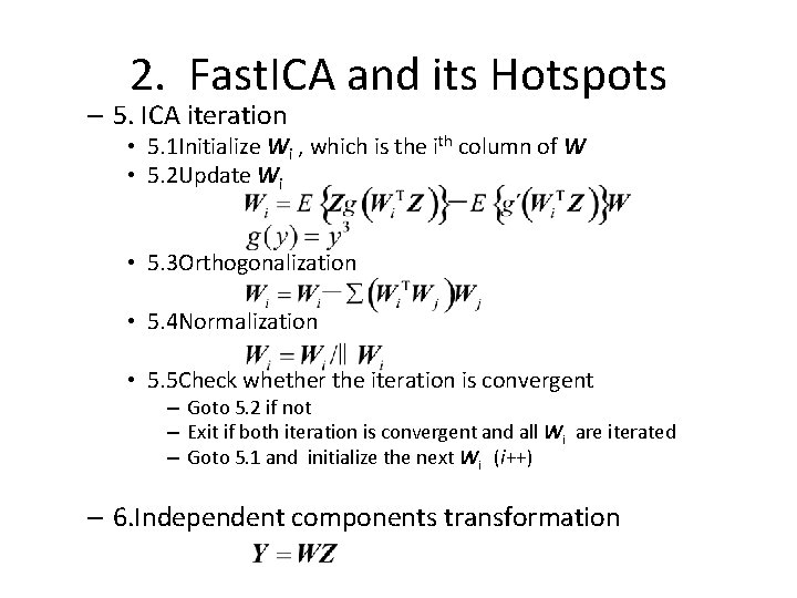
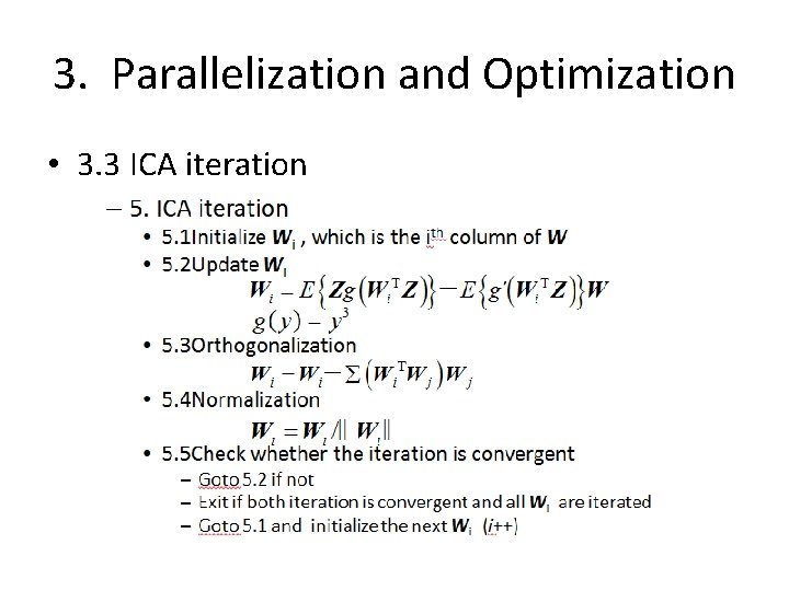
2. Fast. ICA and its Hotspots – 5. ICA iteration • 5. 1 Initialize Wi , which is the ith column of W • 5. 2 Update Wi • 5. 3 Orthogonalization • 5. 4 Normalization • 5. 5 Check whether the iteration is convergent – Goto 5. 2 if not – Exit if both iteration is convergent and all Wi are iterated – Goto 5. 1 and initialize the next Wi (i++) – 6. Independent components transformation

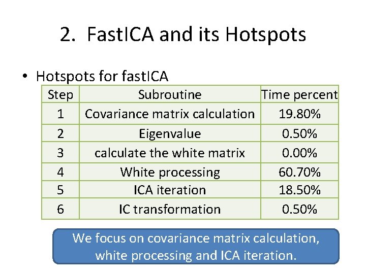
2. Fast. ICA and its Hotspots • Hotspots for fast. ICA Step Subroutine Time percent 1 Covariance matrix calculation 19. 80% 2 Eigenvalue 0. 50% 3 calculate the white matrix 0. 00% 4 White processing 60. 70% 5 ICA iteration 18. 50% 6 IC transformation 0. 50% We focus on covariance matrix calculation, white processing and ICA iteration.

Outline • 1. Motivation • 2. Fast. ICA and its Hotspots • 3. Parallelization and Optimization – – – Covariance matrix calculation White processing ICA iteration • 4. Ms-Fast. ICA and Experimental Result • 5. Conclusions

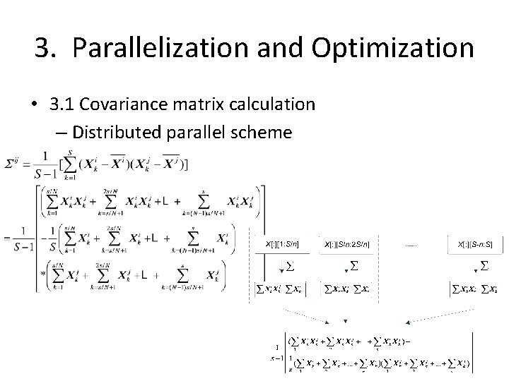
3. Parallelization and Optimization • 3. 1 Covariance matrix calculation – Distributed parallel scheme

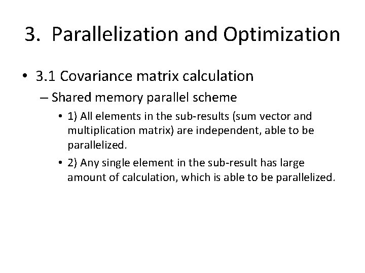
3. Parallelization and Optimization • 3. 1 Covariance matrix calculation – Shared memory parallel scheme • 1) All elements in the sub-results (sum vector and multiplication matrix) are independent, able to be parallelized. • 2) Any single element in the sub-result has large amount of calculation, which is able to be parallelized.

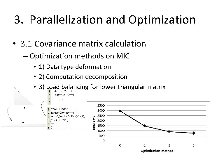
3. Parallelization and Optimization • 3. 1 Covariance matrix calculation – Optimization methods on MIC • 1) Data type deformation • 2) Computation decomposition • 3) Load balancing for lower triangular matrix

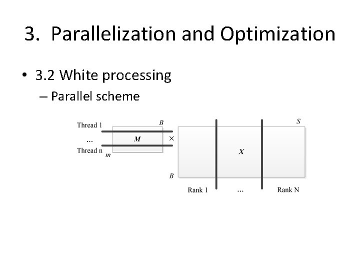
3. Parallelization and Optimization • 3. 2 White processing – Parallel scheme

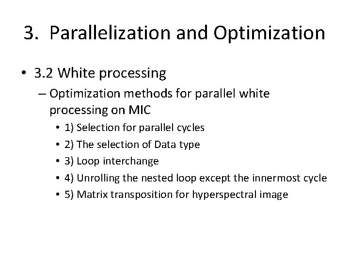
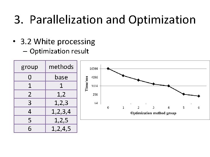
3. Parallelization and Optimization • 3. 2 White processing – Optimization methods for parallel white processing on MIC • • • 1) Selection for parallel cycles 2) The selection of Data type 3) Loop interchange 4) Unrolling the nested loop except the innermost cycle 5) Matrix transposition for hyperspectral image

3. Parallelization and Optimization • 3. 2 White processing – Optimization result group 0 1 2 3 4 5 6 methods base 1 1, 2, 3, 4 1, 2, 5 1, 2, 4, 5

3. Parallelization and Optimization • 3. 3 ICA iteration

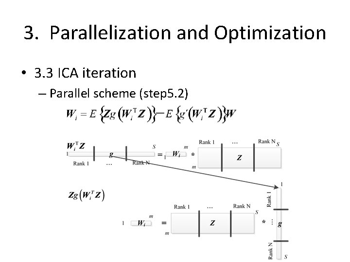
3. Parallelization and Optimization • 3. 3 ICA iteration – Parallel scheme (step 5. 2)

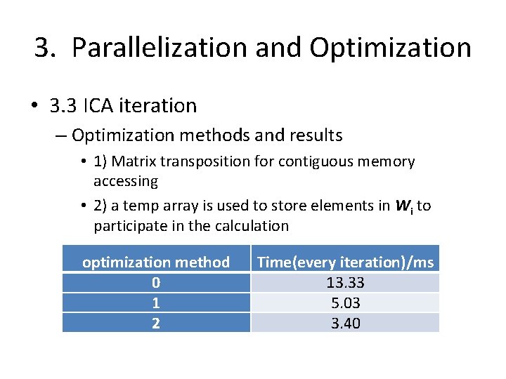
3. Parallelization and Optimization • 3. 3 ICA iteration – Optimization methods and results • 1) Matrix transposition for contiguous memory accessing • 2) a temp array is used to store elements in Wi to participate in the calculation optimization method 0 1 2 Time(every iteration)/ms 13. 33 5. 03 3. 40

Outline • 1. Motivation • 2. Fast. ICA and its Hotspots • 3. Parallelization and Optimization – – – Covariance matrix calculation White processing ICA iteration • 4. Ms-Fast. ICA and Experimental Result • 5. Conclusions

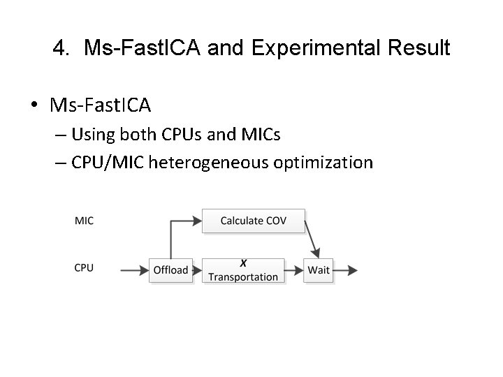
4. Ms-Fast. ICA and Experimental Result • Ms-Fast. ICA – Using both CPUs and MICs – CPU/MIC heterogeneous optimization

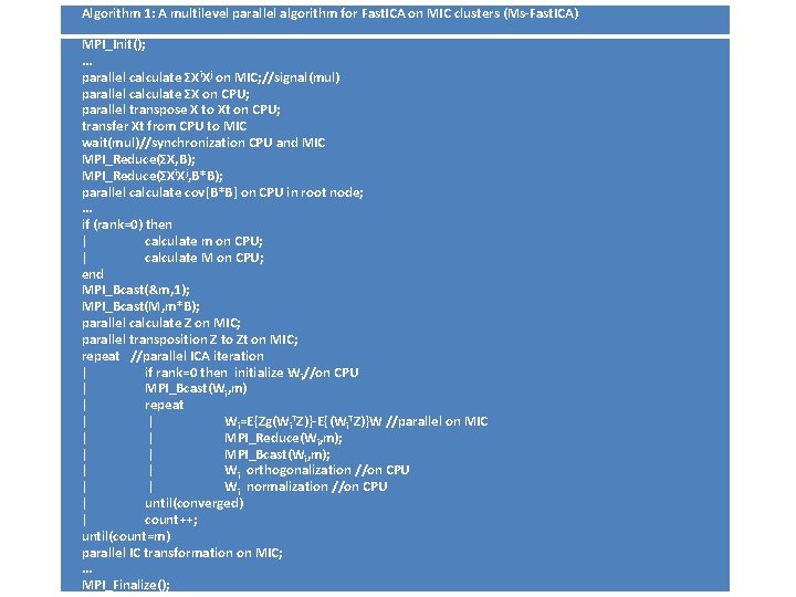
Algorithm 1: A multilevel parallel algorithm for Fast. ICA on MIC clusters (Ms-Fast. ICA) MPI_Init(); . . . parallel calculate ΣX i. Xj on MIC; //signal(mul) parallel calculate ΣX on CPU; parallel transpose X to Xt on CPU; transfer Xt from CPU to MIC wait(mul)//synchronization CPU and MIC MPI_Reduce(ΣX, B); MPI_Reduce(ΣXi. Xj, B*B); parallel calculate cov[B*B] on CPU in root node; . . . if (rank=0) then | calculate m on CPU; | calculate M on CPU; end MPI_Bcast(&m, 1); MPI_Bcast(M, m*B); parallel calculate Z on MIC; parallel transposition Z to Zt on MIC; repeat //parallel ICA iteration | if rank=0 then initialize W i//on CPU | MPI_Bcast(Wi, m) | repeat | | Wi=E{Zg(Wi. TZ)}-E{(Wi. TZ)}W //parallel on MIC | | MPI_Reduce(Wi, m); | | MPI_Bcast(Wi, m); | | Wi orthogonalization //on CPU | | Wi normalization //on CPU | until(converged) | count++; until(count=m) parallel IC transformation on MIC; . . . MPI_Finalize();

4. Ms-Fast. ICA and Experimental Result • Experimental setup – Tianhe-2 Supercomputer • Each node has two 12 -core Intel Xeon CPUs • Each node has three 57 -core Intel Xeon Phi coprocessors – Intel C/C++ compiler 2013 sp 1. 1. 106 • Optimization options “-O 3” – MPICH 3

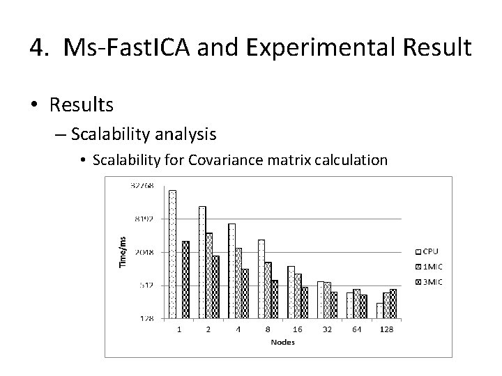
4. Ms-Fast. ICA and Experimental Result • Results – Scalability analysis • Scalability for Covariance matrix calculation

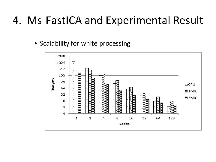
4. Ms-Fast. ICA and Experimental Result • Scalability for white processing

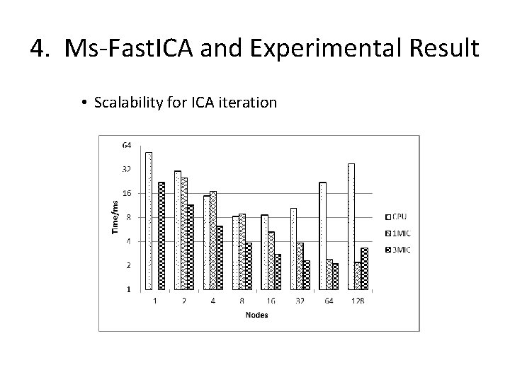
4. Ms-Fast. ICA and Experimental Result • Scalability for ICA iteration

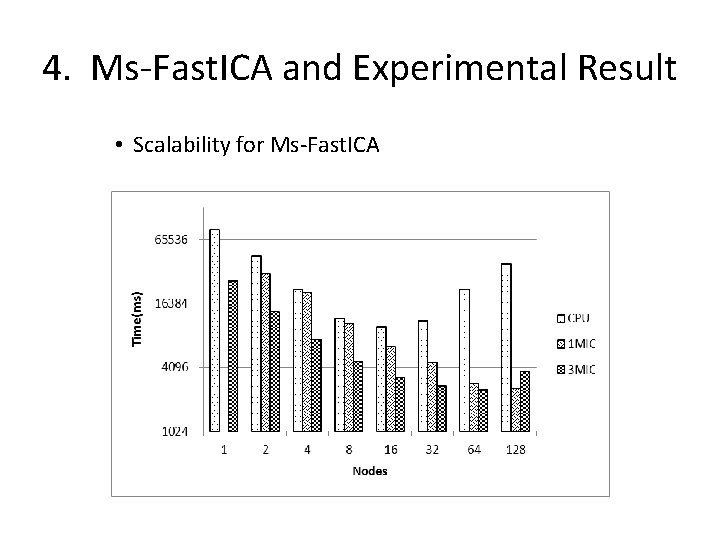
4. Ms-Fast. ICA and Experimental Result • Scalability for Ms-Fast. ICA

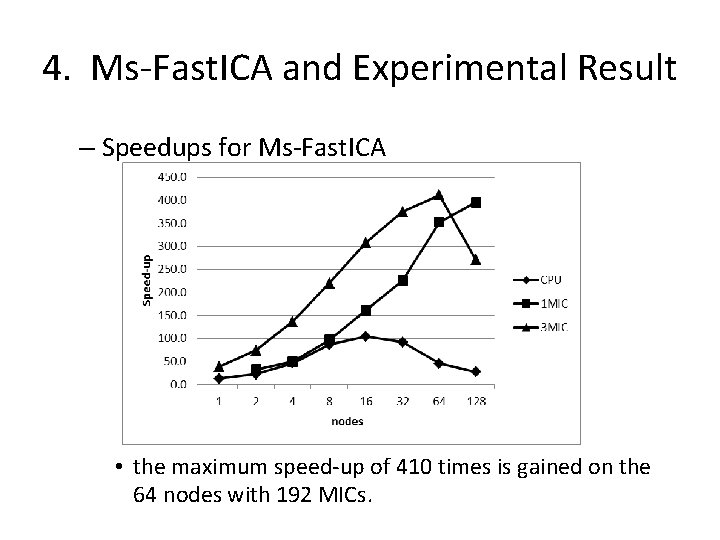
4. Ms-Fast. ICA and Experimental Result – Speedups for Ms-Fast. ICA • the maximum speed-up of 410 times is gained on the 64 nodes with 192 MICs.

Outline • 1. Motivation • 2. Fast. ICA and its Hotspots • 3. Parallelization and Optimization – – – Covariance matrix calculation White processing ICA iteration • 4. Ms-Fast. ICA and Experimental Result • 5. Conclusions

5. Conclusions • Dimensionality reduction is necessary, time is consuming and parallel computing is needed. • By hotspots analysis for Fast. ICA, We focus on covariance matrix calculation, white processing and ICA iteration for parallelized. • We propose the. Parallel schemes and optimization methods for covariance matrix calculation, white processing and ICA iteration. • we implement our work as Ms-Fast. ICA on MIC-based clusters. • Experimental results approve the Ms-Fast. ICA algorithm achieves an excellent scalability. • It can reach a maximum speed-up of 410 times on 64 nodes with 3 MICs per node of the Tianhe-2 Supercomputer.

Thanks! Minquan Fang National University of Defence Technology E-mail: fmq@hpc 6. com