Hidden Markov Models in NLP Leah Spontaneo Introduction

Hidden Markov Models in NLP Leah Spontaneo

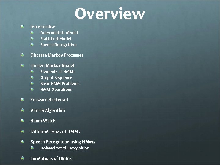
Introduction Overview Deterministic Model Statistical Model Speech Recognition Discrete Markov Processes Hidden Markov Model Elements of HMMs Output Sequence Basic HMM Problems HMM Operations Forward-Backward Viterbi Algorithm Baum-Welch Different Types of HMMs Speech Recognition using HMMs Isolated Word Recognition Limitations of HMMs

Introduction Real-world processes generally produce observable outputs characterized in signals Signals can be discrete or continuous Signal source can be stationary or nonstationary They can be pure or corrupted

Introduction Signals are characterized in signal models Process the signal to provide desired output Learn about the signal source without the source available Work well in practice Signal models can be deterministic or statistical

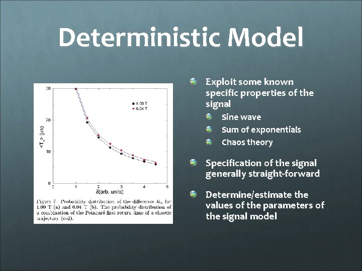
Deterministic Model Exploit some known specific properties of the signal Sine wave Sum of exponentials Chaos theory Specification of the signal generally straight-forward Determine/estimate the values of the parameters of the signal model

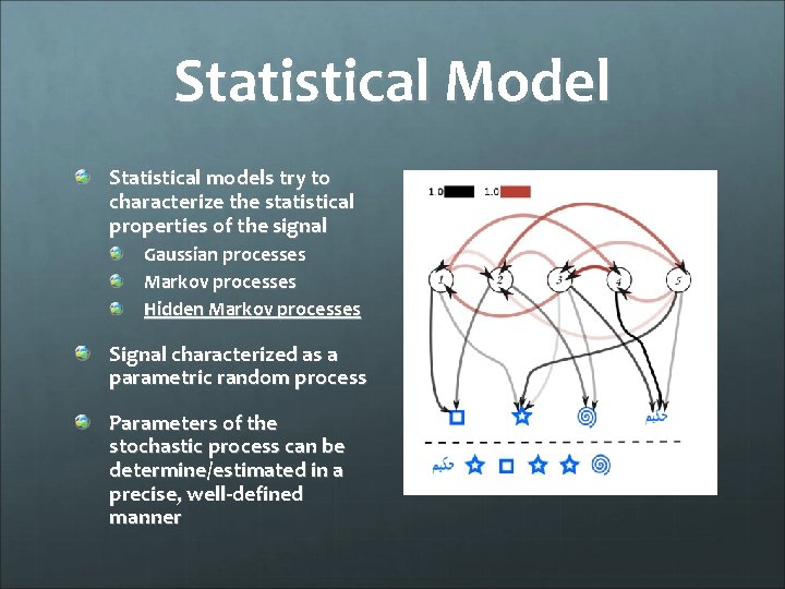
Statistical Model Statistical models try to characterize the statistical properties of the signal Gaussian processes Markov processes Hidden Markov processes Signal characterized as a parametric random process Parameters of the stochastic process can be determine/estimated in a precise, well-defined manner

Speech Recognition Basic theory of hidden Markov models in speech recognition originally pulished in 1960 s by Baum and collegues Implemented in speech processing applications in 1970 s be Baker at CMU and by Jelinek at IBM

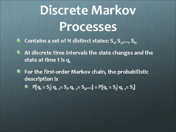
Discrete Markov Processes Contains a set of N distinct states: S 1, S 2, . . . , SN At discrete time intervals the state changes and the state at time t is qt For the first-order Markov chain, the probabilistic description is P[qt = Sj| qt -1= Si, qt -2= Sk, . . . ] = P[qt = Sj| qt -1= Si]

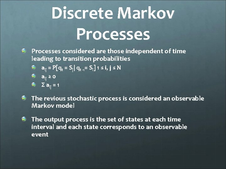
Discrete Markov Processes considered are those independent of time leading to transition probabilities aij = P[qt = Sj| qt -1= Si] 1 ≤ i, j ≤ N aij ≥ 0 Σ aij = 1 The revious stochastic process is considered an observable Markov model The output process is the set of states at each time interval and each state corresponds to an observable event

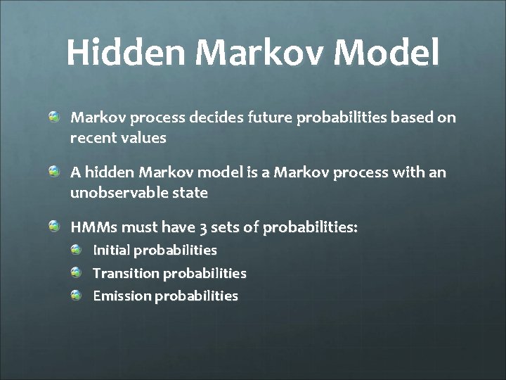
Hidden Markov Model Markov process decides future probabilities based on recent values A hidden Markov model is a Markov process with an unobservable state HMMs must have 3 sets of probabilities: Initial probabilities Transition probabilities Emission probabilities

Hidden Markov Model Includes the case where the observation is a probabilistic function of the state A doubly embedded stochastic process with an underlying unobservable stochastic process Unobservable process only observed through a set of stochastic processes producing the observations

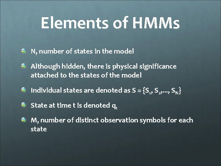
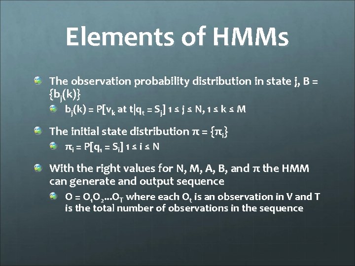
Elements of HMMs N, number of states in the model Although hidden, there is physical significance attached to the states of the model Individual states are denoted as S = {S 1, S 2, . . . , SN} State at time t is denoted qt M, number of distinct observation symbols for each state

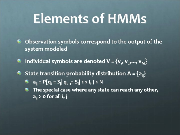
Elements of HMMs Observation symbols correspond to the output of the system modeled Individual symbols are denoted V = {v 1, v 2, . . . , v. M} State transition probability distribution A = {aij} aij = P[qt = Sj| qt -1= Si] 1 ≤ i, j ≤ N The special case where any state can reach any other, aij > 0 for all i, j

Elements of HMMs The observation probability distribution in state j, B = {bj(k)} bj(k) = P[vk at t|qt = Sj] 1 ≤ j ≤ N, 1 ≤ k ≤ M The initial state distribution π = {πi} πi = P[q 1 = Si] 1 ≤ i ≤ N With the right values for N, M, A, B, and π the HMM can generate and output sequence O = O 1 O 2. . . OT where each Ot is an observation in V and T is the total number of observations in the sequence

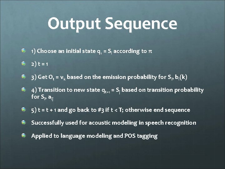
Output Sequence 1) Choose an initial state q 1 = Si according to π 2) t = 1 3) Get Ot = vk based on the emission probability for Si, bi(k) 4) Transition to new state qt+1 = Sj based on transition probability for Si, aij 5) t = t + 1 and go back to #3 if t < T; otherwise end sequence Successfully used for acoustic modeling in speech recognition Applied to language modeling and POS tagging

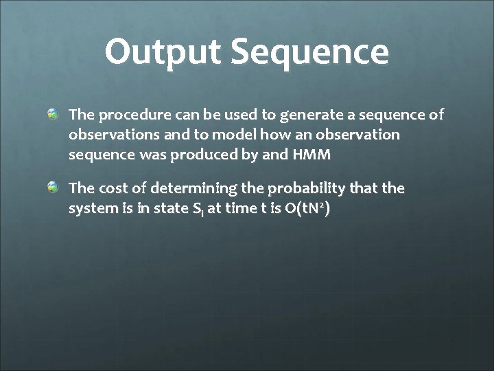
Output Sequence The procedure can be used to generate a sequence of observations and to model how an observation sequence was produced by and HMM The cost of determining the probability that the system is in state Si at time t is O(t. N 2)

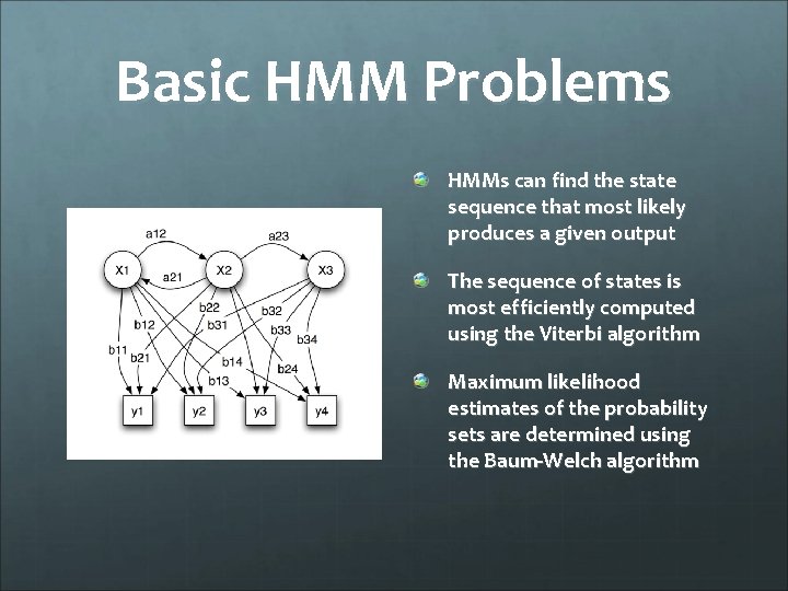
Basic HMM Problems HMMs can find the state sequence that most likely produces a given output The sequence of states is most efficiently computed using the Viterbi algorithm Maximum likelihood estimates of the probability sets are determined using the Baum-Welch algorithm

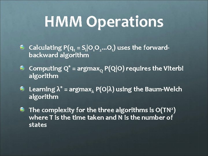
HMM Operations Calculating P(qt = Si|O 1 O 2. . . Ot) uses the forwardbackward algorithm Computing Q* = argmax. Q P(Q|O) requires the Viterbi algorithm Learning λ* = argmaxλ P(O|λ) using the Baum-Welch algorithm The complexity for the three algorithms is O(TN 2) where T is the time taken and N is the number of states

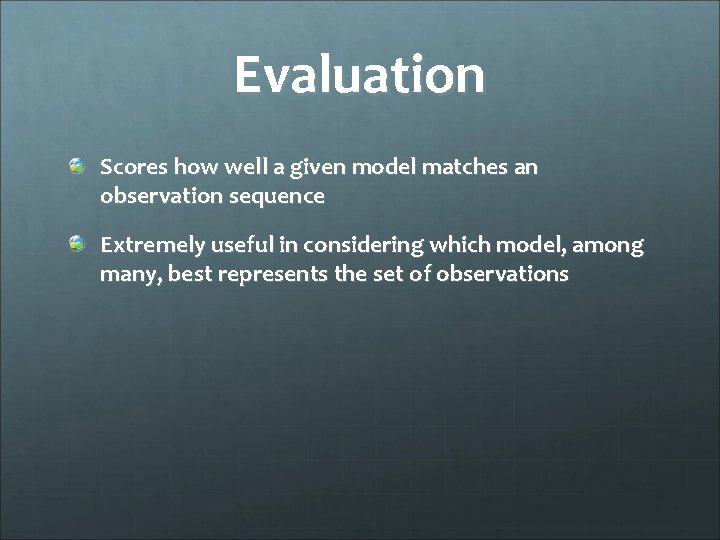
Evaluation Scores how well a given model matches an observation sequence Extremely useful in considering which model, among many, best represents the set of observations

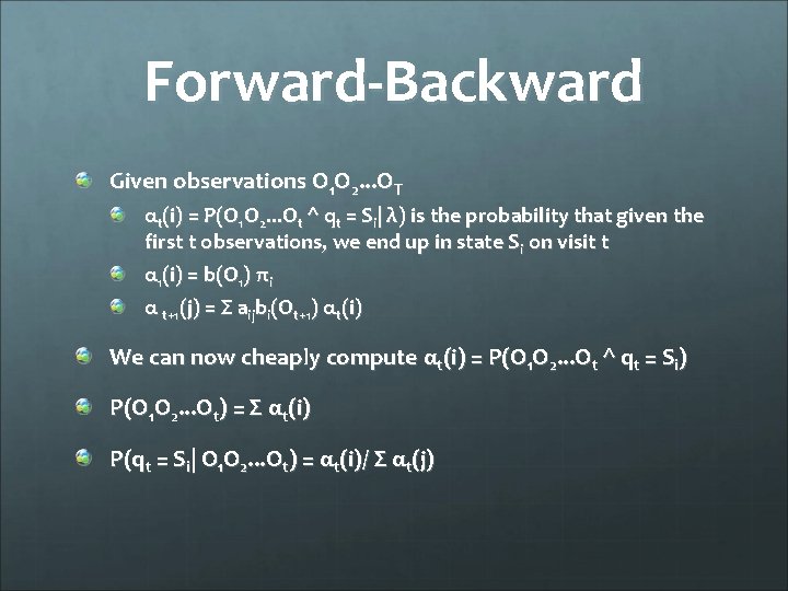
Forward-Backward Given observations O 1 O 2. . . OT αt(i) = P(O 1 O 2. . . Ot ^ qt = Si| λ) is the probability that given the first t observations, we end up in state Si on visit t α 1(i) = b(O 1) πi α t+1(j) = Σ aijbi(Ot+1) αt(i) We can now cheaply compute αt(i) = P(O 1 O 2. . . Ot ^ qt = Si) P(O 1 O 2. . . Ot) = Σ αt(i) P(qt = Si| O 1 O 2. . . Ot) = αt(i)/ Σ αt(j)

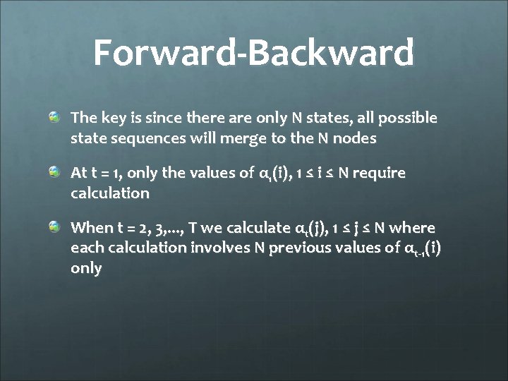
Forward-Backward The key is since there are only N states, all possible state sequences will merge to the N nodes At t = 1, only the values of α 1(i), 1 ≤ i ≤ N require calculation When t = 2, 3, . . . , T we calculate αt(j), 1 ≤ j ≤ N where each calculation involves N previous values of αt-1(i) only

State Sequence There is no ‘correct’ state sequence except for degenerate models Optimality criterion is used instead to determine the best possible outcome There are several reasonable optimality criteria and thus, the chosen criterion depends on the use of the uncovered sequence Used for continuous speech recognition

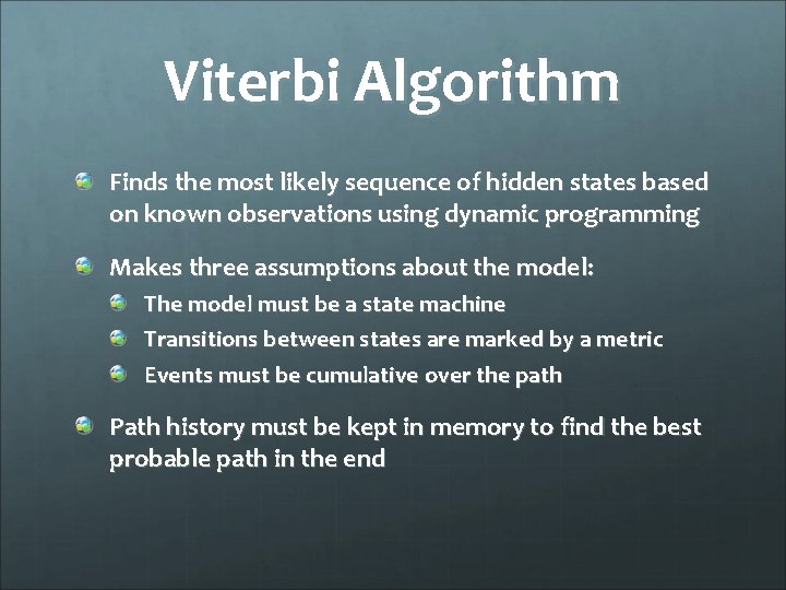
Viterbi Algorithm Finds the most likely sequence of hidden states based on known observations using dynamic programming Makes three assumptions about the model: The model must be a state machine Transitions between states are marked by a metric Events must be cumulative over the path Path history must be kept in memory to find the best probable path in the end

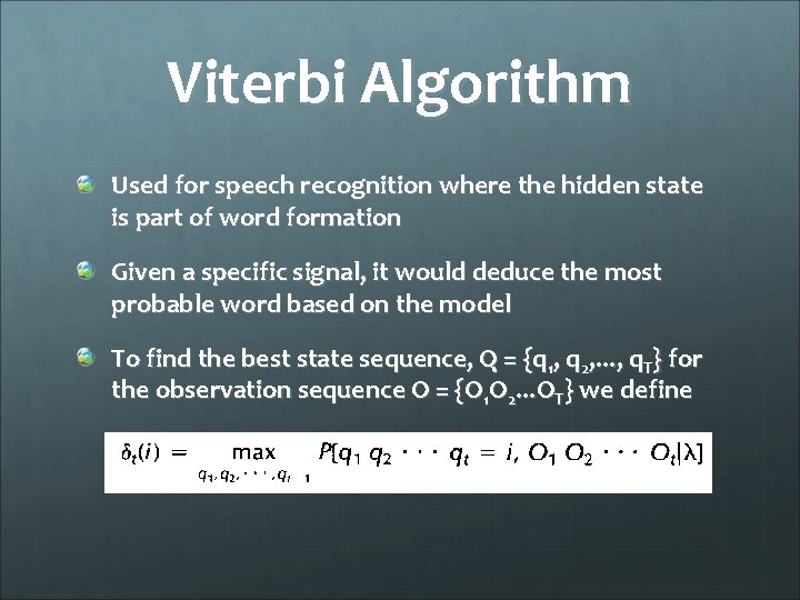
Viterbi Algorithm Used for speech recognition where the hidden state is part of word formation Given a specific signal, it would deduce the most probable word based on the model To find the best state sequence, Q = {q 1, q 2, . . . , q. T} for the observation sequence O = {O 1 O 2. . . OT} we define

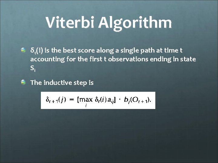
Viterbi Algorithm δt(i) is the best score along a single path at time t accounting for the first t observations ending in state Si The inductive step is

Viterbi Algorithm Similar to forward calculation of the forwardbackward algorithm The major difference is the maximization over the previous states instead of summing the probabilities

Optimizing Parameters A training sequence is used to train the HMM and adjust the model parameters Training problem is crucial for most HMM applications Allows us to optimally adapt model parameters to observed training data creating good models for real data

Baum-Welch A special case of expectation maximization EM has two main steps: Devise the expectation of the log-likelihood using current estimates of latent variables Compute the maximized log-likelihood using values from the first step Baum-Welch is a form of generalized EM which allows the algorithm to converge to a local optimum

Baum-Welch Also known as the forward-backwards algorithm Baum-Welch uses two main steps: The forward and backward probability is calculated for each state in the HMM The transition and emission probabilities are determined and divided by the probability of the whole model based on the previous step

Baum-Welch Cons: lots of local minima Pros: local minima are often adequate models of the data EM requires the number of states to be given Sometimes HMMs require some links to be zero. For this aij = 0 in the initial estimate λ(0)

Different Types of HMM Left-right model As time increases the state index increases or stays the same No transitions are allowed between states whose indecies are lower than the current state Cross-coupled two parallel left-right Obeys the left-right constraints on transition probabilities but provide more flexibility

Speech Recognition using HMMs Feature Analysis: A spectral/temporal analysis of speech signals can be performed to provide observation vectors used to train HMMs Unit Matching: Each unit is characterized by an HMM with parameters estimated from speech data Provides the likelihoods of matches of all sequences of speech recognition units to the unknown input

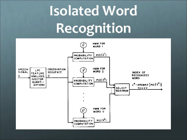
Isolated Word Recognition Vocabulary of V words to be recognized and each modeled by a distinct HMM For each word, a training set of K occurrences of each spoken word where each occurrence of the word is an observation sequence For each word v, build an HMM (estimating the model parameters which optimize the likelihood of the training set observations for each word)

Isolated Word Recognition For each unknown word recognized, measure the observation sequence O = {O 1 O 2. . . OT} via feature analysis of the speech corresponding to the word Calculate model likelihoods for all possible models followed by the selection of the word with the highest model likelihood

Isolated Word Recognition

Limitations of HMMs Assumption that successive observations are independent and thus, the probability of an observation sequence can be written as the product of the probabilities of individual observations Assumes the distributions of individual observation parameters are well represented as a mixture of autoregressive or Gaussian densities Assumption of being in a given state at each time interval inappropriate for speech sound which can extend through several states

Questions?

References Vogel, S. , et al. “HMM-based word alignment in statistical translation. ” In Proceedings of the 16 th conference on Computational linguistics (1996), pp. 836 -841. Rabiner, L. R. “A Tutorial on Hidden Markov Models and Selected Applications in Speech Recognition. ” Proceedings of the IEEE (1989), pp. 257 -286. Moore, A. W. “Hidden Markov Models. ” Carnegie Mellon University. https: //wiki. cse. yorku. ca/course_archive/201011/F/6390/_media/hmm 14. pdf http: //en. wikipedia. org/wiki/Hidden_Markov_model