Graphs 15 211 Fundamental Data Structures and Algorithms

Graphs 15 -211 Fundamental Data Structures and Algorithms Ananda Gunawardena April 4, 2006

In this lecture § concept § Representations ØAdjacency matrix ØAdjacency List § Graph Traversals ØBFS, DFS § Minimum Spanning Trees § Search Engines

Introduction to Graphs

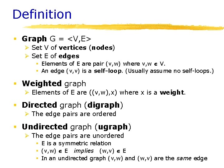
Definition § Graph G = <V, E> Ø Set V of vertices (nodes) Ø Set E of edges § Elements of E are pair (v, w) where v, w V. § An edge (v, v) is a self-loop. (Usually assume no self-loops. ) § Weighted graph Ø Elements of E are ((v, w), x) where x is a weight. § Directed graph (digraph) Ø The edge pairs are ordered § Undirected graph (ugraph) Ø The edge pairs are unordered § E is a symmetric relation § (v, w) E implies (w, v) E § In an undirected graph (v, w) and (w, v) are the same edge

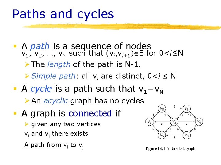
Paths and cycles § A path is a sequence of nodes v 1, v 2, …, v. N such that (vi, vi+1) E for 0<i≤N Ø The length of the path is N-1. Ø Simple path: all vi are distinct, 0<i ≤ N § A cycle is a path such that v 1=v. N Ø An acyclic graph has no cycles § A graph is connected if Ø given any two vertices vi and vj there exists A path from vi to vj figure 14. 1 A directed graph

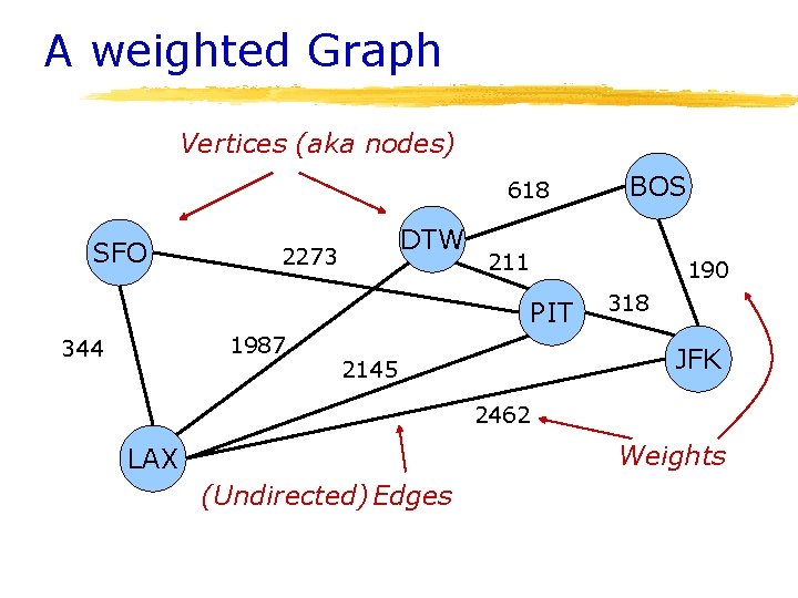
A weighted Graph Vertices (aka nodes) 618 SFO DTW 2273 211 190 PIT 1987 344 BOS 318 JFK 2145 2462 Weights LAX (Undirected) Edges

Applications of directed graphs § Many of the common applications of graphs use directed graphs. § Often this occurs when the edges represent an asymmetric relationship. ØE. g. , the inheritance relationship between classes. ØE. g. , scheduling constraints.

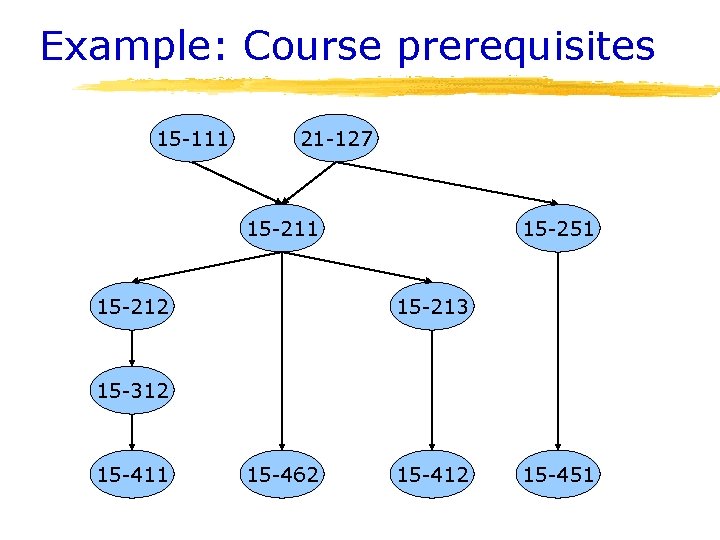
Example: Course prerequisites 15 -111 21 -127 15 -211 15 -212 15 -251 15 -213 15 -312 15 -411 15 -462 15 -412 15 -451

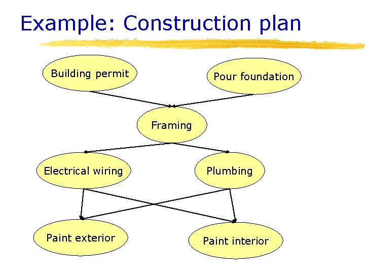
Example: Construction plan Building permit Pour foundation Framing Electrical wiring Paint exterior Plumbing Paint interior

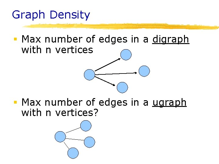
Graph Density § Max number of edges in a digraph with n vertices § Max number of edges in a ugraph with n vertices?

Dense Graphs vs Sparse Graphs § A dense graph is a graph where the number of edges is relatively large compared to number of nodes § When is a graph a dense graph? Ø We could use § |E| = O(|V|2) - Dense § |E| = O(|V|) - Sparse § Examples of Ø Dense Graphs § Each node is connected to at least 25% of other nodes Ø Sparse Graphs § Each node is connected to only a constant number of other nodes

Relevance of a Node § Suppose G =<V, E> is a digraph and u is a vertex in V. Then § indegree(u) = {v | (v, u) in E} ØThat is, number of links into node u § outdegree(u) = {v | (u, v) in E} Øi. e. number of links out of u

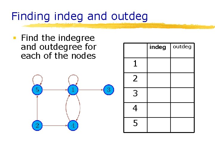
Finding indeg and outdeg § Find the indegree and outdegree for each of the nodes indeg 1 2 3 4 5 outdeg

Graph Representations

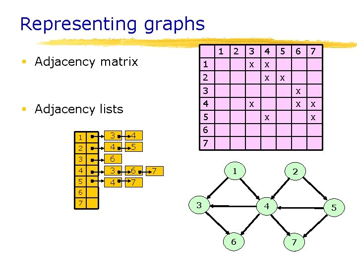
Representing graphs 1 § Adjacency matrix 1 2 3 4 5 6 7 § Adjacency lists 4 5 4 3 4 6 3 5 4 7 1 2 3 6 2 3 x 4 x x 6 x 7 x x 1 7 5 x x 2 6 7 3 4 6 5 7

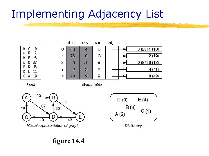
Implementing Adjacency List figure 14. 4

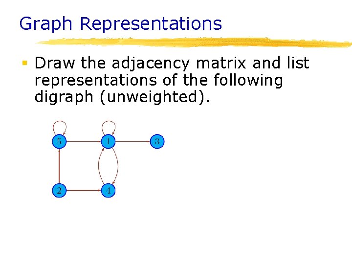
Graph Representations § Draw the adjacency matrix and list representations of the following digraph (unweighted).

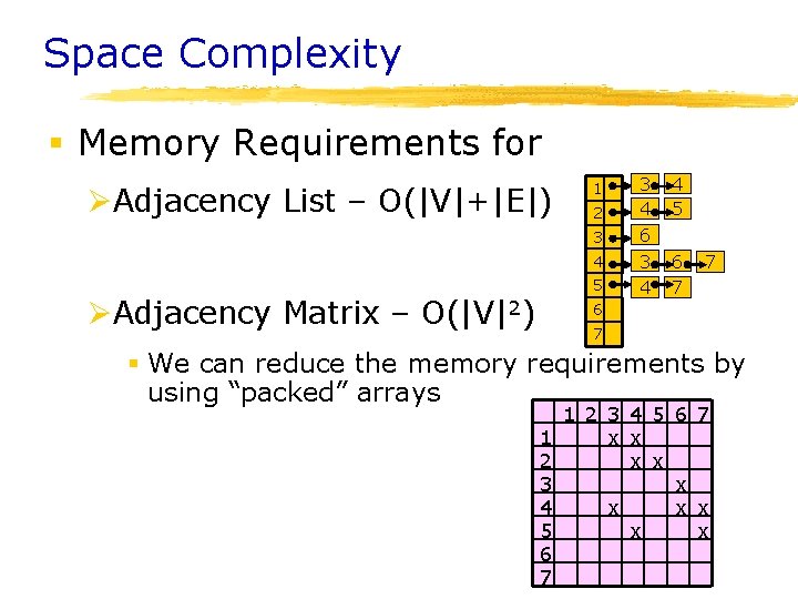
Space Complexity § Memory Requirements for ØAdjacency List – O(|V|+|E|) 1 2 3 4 ØAdjacency Matrix – O(|V|2) 5 3 4 6 3 4 4 5 6 7 7 6 7 § We can reduce the memory requirements by using “packed” arrays 1 2 3 4 5 6 7 1 x x 2 x x 3 x 4 x x x 5 x x 6 7

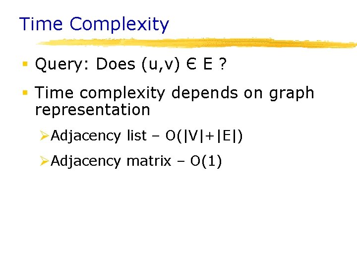
Time Complexity § Query: Does (u, v) Є E ? § Time complexity depends on graph representation ØAdjacency list – O(|V|+|E|) ØAdjacency matrix – O(1)

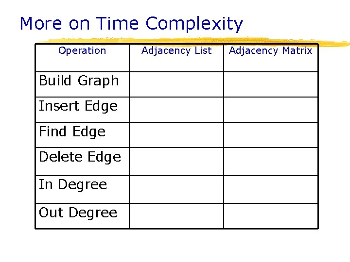
More on Time Complexity Operation Build Graph Insert Edge Find Edge Delete Edge In Degree Out Degree Adjacency List Adjacency Matrix

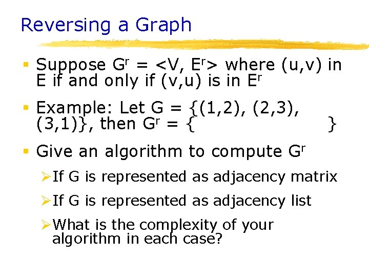
Reversing a Graph § Suppose Gr = <V, Er> where (u, v) in E if and only if (v, u) is in Er § Example: Let G = {(1, 2), (2, 3), (3, 1)}, then Gr = { } § Give an algorithm to compute Gr ØIf G is represented as adjacency matrix ØIf G is represented as adjacency list ØWhat is the complexity of your algorithm in each case?

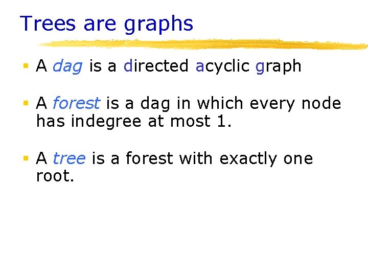
Trees are graphs § A dag is a directed acyclic graph § A forest is a dag in which every node has indegree at most 1. § A tree is a forest with exactly one root.

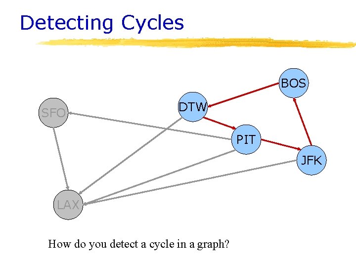
Detecting Cycles BOS SFO DTW PIT JFK LAX How do you detect a cycle in a graph?

Reachability

Reachability § Given a node u in V, find all the nodes v in V that are reachable from u. That is, find the set Ø R(u) = {v|There is a path from u to v} § How do we compute R(u)? Ø u is in R(u) – trivial or base case Ø If v is in R(u) and (v, z) in E, then z is in R(u) § So we can inductively find the set R(u)

Reachability Algorithms § There are two algorithms ØDepth First Search (DFS) § Explore the nodes by going deeper and deeper into the graph. Use back tracking to try different paths (uses a stack) ØBreadth First Search (BFS) § Explore the nodes in an orderly manner. Look at the nodes that are closest to source. Then look at their neighbors, etc. . (uses a queue)

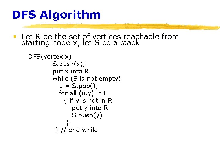
DFS Algorithm § Let R be the set of vertices reachable from starting node x, let S be a stack DFS(vertex x) S. push(x); put x into R while (S is not empty) u = S. pop(); for all (u, y) in E { if y is not in R put y into R S. push(y) } } // end while

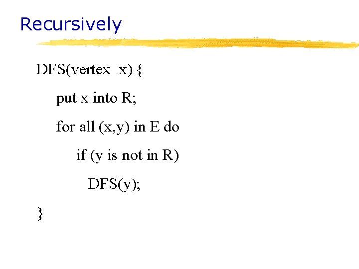
Recursively DFS(vertex x) { put x into R; for all (x, y) in E do if (y is not in R) DFS(y); }

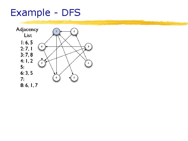
Example - DFS

Finding Cycles in a Graph

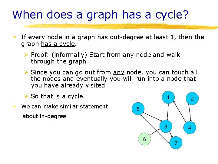
When does a graph has a cycle? § If every node in a graph has out-degree at least 1, then the graph has a cycle. Ø Proof: (informally) Start from any node and walk through the graph Ø Since you can go out from any node, you can touch all the nodes and eventually you will run into a node that you have already visited. Ø So that is a cycle. § We can make similar statement about in-degree

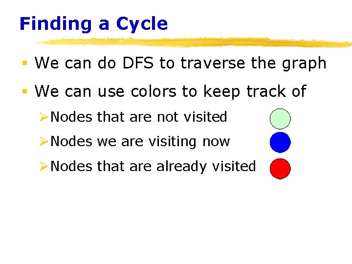
Finding a Cycle § We can do DFS to traverse the graph § We can use colors to keep track of ØNodes that are not visited ØNodes we are visiting now ØNodes that are already visited

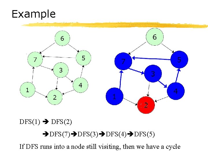
Example DFS(1) DFS(2) DFS(7) DFS(3) DFS(4) DFS(5) If DFS runs into a node still visiting, then we have a cycle

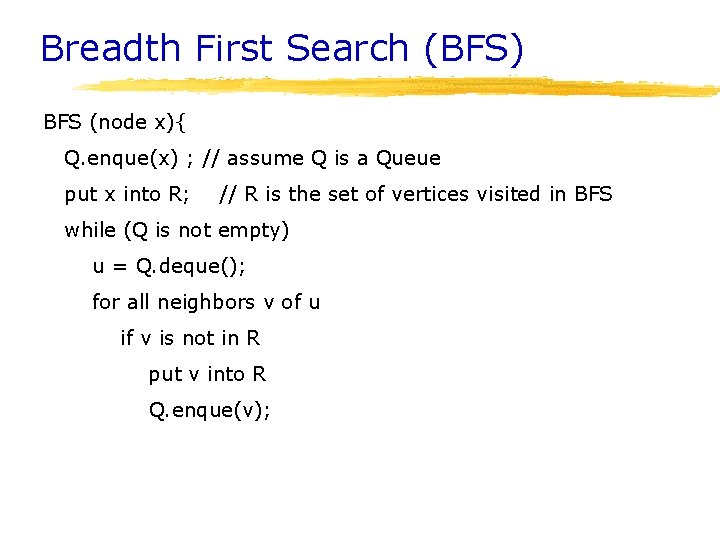
Breadth First Search (BFS) BFS (node x){ Q. enque(x) ; // assume Q is a Queue put x into R; // R is the set of vertices visited in BFS while (Q is not empty) u = Q. deque(); for all neighbors v of u if v is not in R put v into R Q. enque(v);

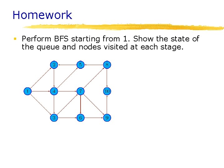
Homework § Perform BFS starting from 1. Show the state of the queue and nodes visited at each stage.

Minimum Spanning Trees

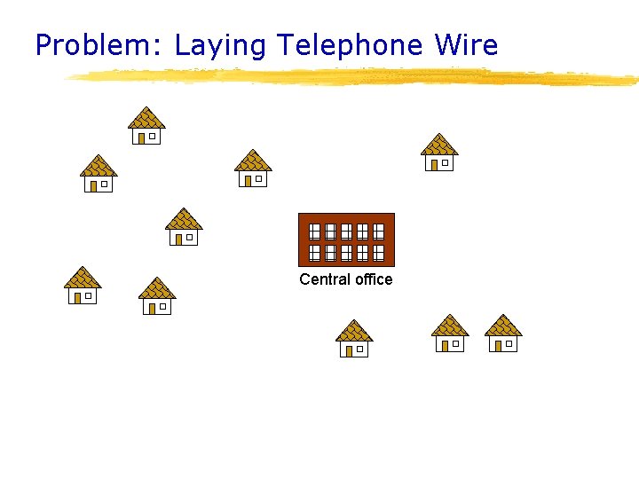
Problem: Laying Telephone Wire Central office

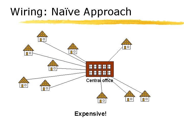
Wiring: Naïve Approach Central office Expensive!

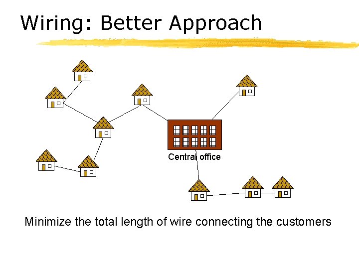
Wiring: Better Approach Central office Minimize the total length of wire connecting the customers

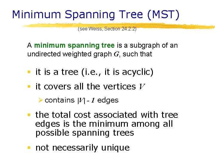
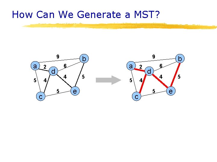
Minimum Spanning Tree (MST) (see Weiss, Section 24. 2. 2) A minimum spanning tree is a subgraph of an undirected weighted graph G, such that § it is a tree (i. e. , it is acyclic) § it covers all the vertices V Ø contains |V| - 1 edges § the total cost associated with tree edges is the minimum among all possible spanning trees § not necessarily unique

How Can We Generate a MST? 9 a 2 5 4 c b 6 d 4 5 5 e

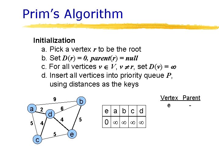
Prim’s Algorithm Initialization a. Pick a vertex r to be the root b. Set D(r) = 0, parent(r) = null c. For all vertices v V, v r, set D(v) = d. Insert all vertices into priority queue P, using distances as the keys 9 a 2 5 4 c b 6 d e a b c d 4 5 5 e 0 Vertex Parent e -

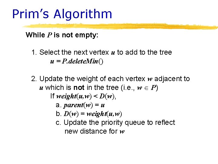
Prim’s Algorithm While P is not empty: 1. Select the next vertex u to add to the tree u = P. delete. Min() 2. Update the weight of each vertex w adjacent to u which is not in the tree (i. e. , w P) If weight(u, w) < D(w), a. parent(w) = u b. D(w) = weight(u, w) c. Update the priority queue to reflect new distance for w

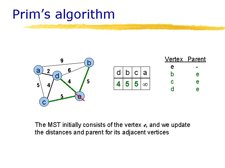
Prim’s algorithm 9 a 2 5 4 c b 6 d d b c a 4 5 5 e 4 5 5 Vertex Parent e b e c e d e The MST initially consists of the vertex e, and we update the distances and parent for its adjacent vertices

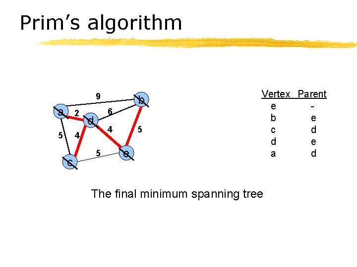
Prim’s algorithm 9 a 2 5 4 c b 6 d 4 5 5 e Vertex Parent e b e c d d e a d The final minimum spanning tree

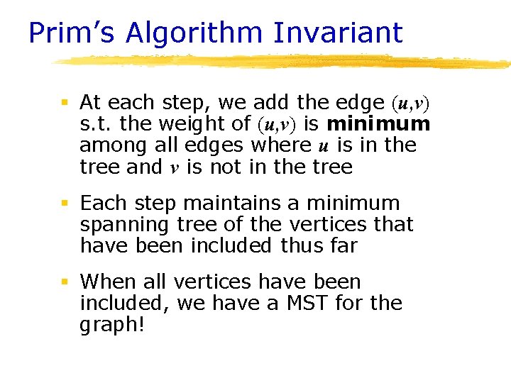
Prim’s Algorithm Invariant § At each step, we add the edge (u, v) s. t. the weight of (u, v) is minimum among all edges where u is in the tree and v is not in the tree § Each step maintains a minimum spanning tree of the vertices that have been included thus far § When all vertices have been included, we have a MST for the graph!

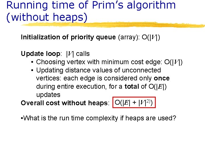
Running time of Prim’s algorithm (without heaps) Initialization of priority queue (array): O(|V|) Update loop: |V| calls • Choosing vertex with minimum cost edge: O(|V|) • Updating distance values of unconnected vertices: each edge is considered only once during entire execution, for a total of O(|E|) updates Overall cost without heaps: O(|E| + |V|2)) • What is the run time complexity if heaps are used?

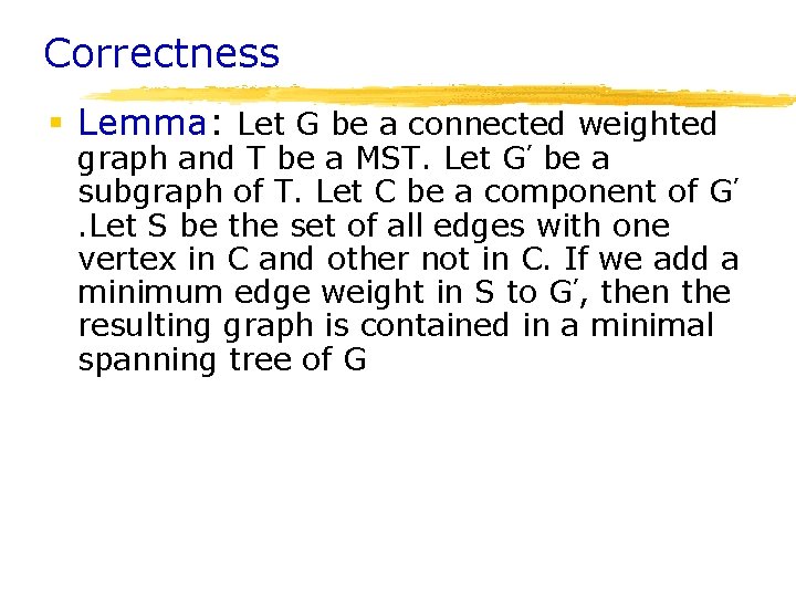
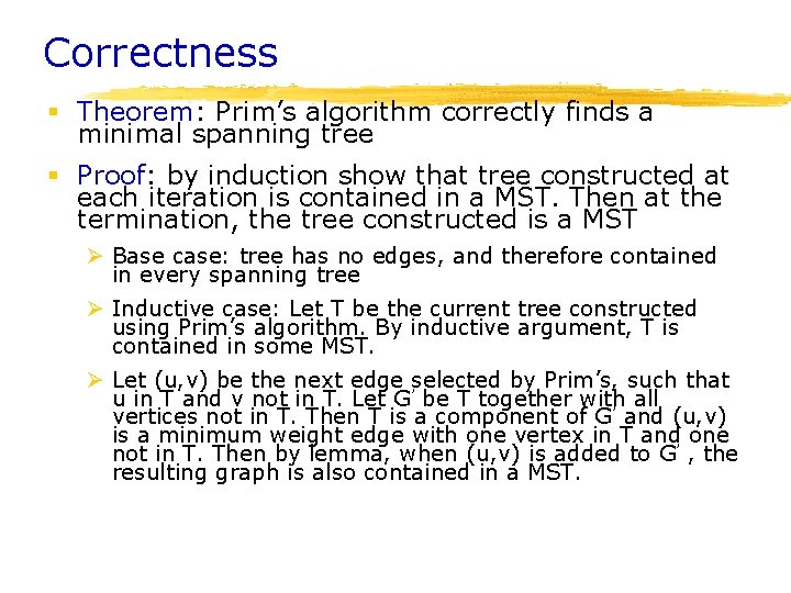
Correctness § Lemma: Let G be a connected weighted graph and T be a MST. Let G’ be a subgraph of T. Let C be a component of G’. Let S be the set of all edges with one vertex in C and other not in C. If we add a minimum edge weight in S to G’, then the resulting graph is contained in a minimal spanning tree of G

Correctness § Theorem: Prim’s algorithm correctly finds a minimal spanning tree § Proof: by induction show that tree constructed at each iteration is contained in a MST. Then at the termination, the tree constructed is a MST Ø Base case: tree has no edges, and therefore contained in every spanning tree Ø Inductive case: Let T be the current tree constructed using Prim’s algorithm. By inductive argument, T is contained in some MST. Ø Let (u, v) be the next edge selected by Prim’s, such that u in T and v not in T. Let G’ be T together with all vertices not in T. Then T is a component of G’ and (u, v) is a minimum weight edge with one vertex in T and one not in T. Then by lemma, when (u, v) is added to G’ , the resulting graph is also contained in a MST.

Web Search Engines A Cool Application of Graphs

Building a Search Engine § Crawl the web § Build a web index § Then we build/search, we may have to sort the index ØGoogle sorts more than 100 billion index items § Novel algorithms, novel data structures, distributed computing

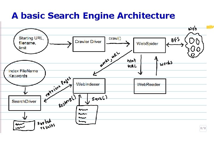
A basic Search Engine Architecture

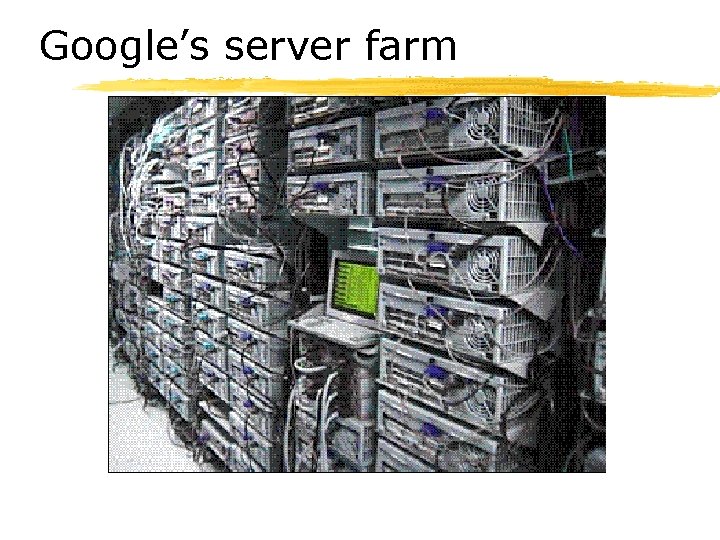
Google’s server farm

Web Crawlers § Start with an initial page P 0. Find URLs on P 0 and add them to a queue § When done with P 0, pass it to an indexing program, get a page P 1 from the queue and repeat § Can be specialized (e. g. only look for email addresses) § Issues Ø Which page to look at next? (Special subjects, recency) Ø How deep within a site do you go (depth search)? Ø How frequently to visit pages?

So, why Spider the Web? § Refresh Collection by deleting dead links Ø OK if index is slightly smaller Ø Done every 1 -2 weeks in best engines § Finding new sites Ø Respider the entire web Ø Done every 2 -4 weeks in best engines

Cost of Spidering § Spider can (and does) run in parallel on hundreds of severs § Very high network connectivity (e. g. T 3 line) § Servers can migrate from spidering to query processing depending on time-of-day load § Running a full web spider takes days even with hundreds of dedicated servers

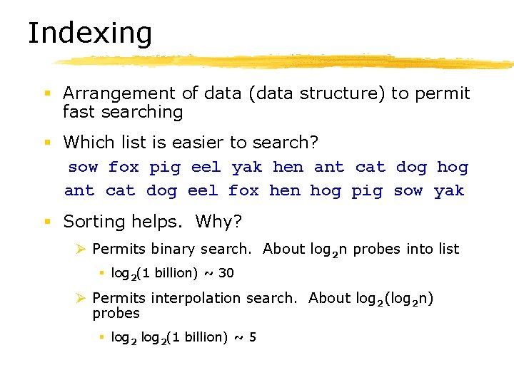
Indexing § Arrangement of data (data structure) to permit fast searching § Which list is easier to search? sow fox pig eel yak hen ant cat dog hog ant cat dog eel fox hen hog pig sow yak § Sorting helps. Why? Ø Permits binary search. About log 2 n probes into list § log 2(1 billion) ~ 30 Ø Permits interpolation search. About log 2(log 2 n) probes § log 2(1 billion) ~ 5

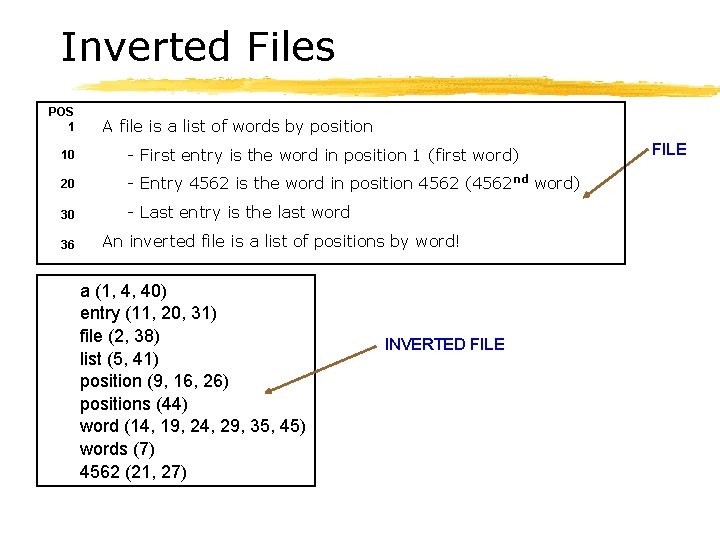
Inverted Files POS 1 A file is a list of words by position 10 - First entry is the word in position 1 (first word) 20 - Entry 4562 is the word in position 4562 (4562 nd word) 30 - Last entry is the last word 36 An inverted file is a list of positions by word! a (1, 4, 40) entry (11, 20, 31) file (2, 38) list (5, 41) position (9, 16, 26) positions (44) word (14, 19, 24, 29, 35, 45) words (7) 4562 (21, 27) INVERTED FILE

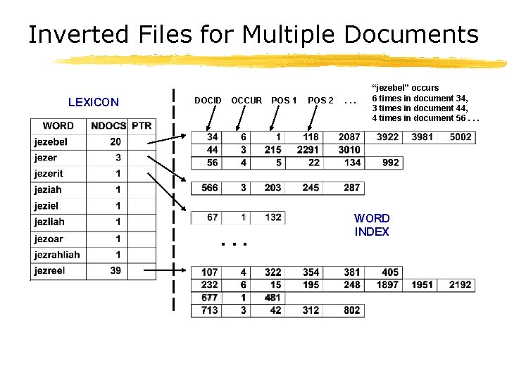
Inverted Files for Multiple Documents LEXICON DOCID OCCUR . . . POS 1 POS 2 . . . “jezebel” occurs 6 times in document 34, 3 times in document 44, 4 times in document 56. . . WORD INDEX

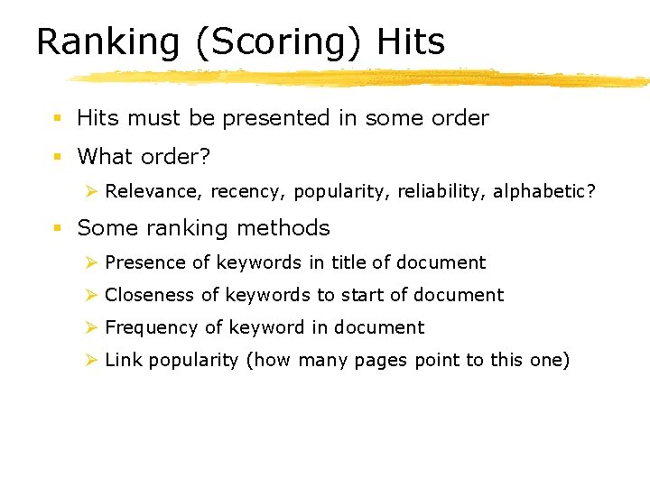
Ranking (Scoring) Hits § Hits must be presented in some order § What order? Ø Relevance, recency, popularity, reliability, alphabetic? § Some ranking methods Ø Presence of keywords in title of document Ø Closeness of keywords to start of document Ø Frequency of keyword in document Ø Link popularity (how many pages point to this one)