15 211 Fundamental Data Structures and Algorithms KMP

15 -211 Fundamental Data Structures and Algorithms KMP Algorithm March 28, 2006 Ananda Gunawardena

String Matching

The Problem • Given a text T and a pattern P, check whether P occurs in T – eg: T = {aabbcbbcabbbcbccccabbabbccc} – Find all occurrences of pattern P = bbc • There are variations of pattern matching – Finding “approximate” matching – Finding multiple patterns etc…. – Searching for multiple patterns etc. .

Why String Matching? • Applications in Computational Biology – DNA sequence is a long word (or text) over a 4 -letter alphabet – GTTTGAGTGGTCAGTCTTTTCGACGGAGCCCCCAATT AATAAACTCATAAGCAGACCTCAGTTCGCTTAGAGCAGCCG AAA…. . – Find a Specific pattern W • Finding patterns in documents formed using a large alphabet – Word processing – Web searching – Desktop search (Google, MSN) • Matching strings of bytes containing – Graphical data – Machine code • grep in unix – grep searches for lines matching a pattern.

String Matching • Text string T[0. . N-1] T = “abacaabaccabaabb” • Pattern string P[0. . M-1] P = “abacab” • Where is the first instance of P in T? T[10. . 15] = P[0. . 5] • Typically N >>> M

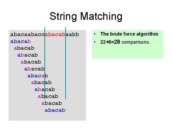
String Matching abacaabaccabaabb abacab abacab abacab • The brute force algorithm • 22+6=28 comparisons.

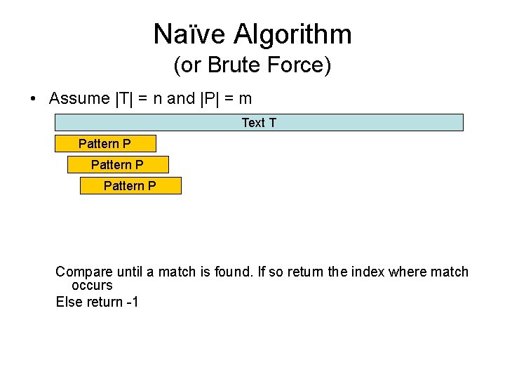
Naïve Algorithm (or Brute Force) • Assume |T| = n and |P| = m Text T Pattern P Compare until a match is found. If so return the index where match occurs Else return -1

Brute Force Version 1 static int match(char[] T, char[] P){ for (int i=0; i<T. length; i++){ boolean flag = true; if (P[0]==T[i]) for (int j=1; j<P. length; j++) if (T[i+j]!=P[j]) {flag=false; break; } if (flag) return i; } } • What is the complexity of the code?

Brute Force, Version 2 static int match(char[] T, char[] P){ // rewrite the brute-force code with only one loop }

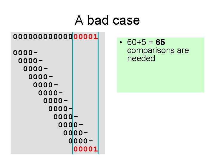
A bad case 000000001 000000000000000000000000001 • 60+5 = 65 comparisons are needed • How many of them could be avoided?

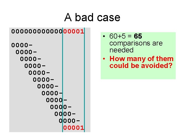
A bad case 000000001 000000000000000000000000001 • 60+5 = 65 comparisons are needed • How many of them could be avoided?

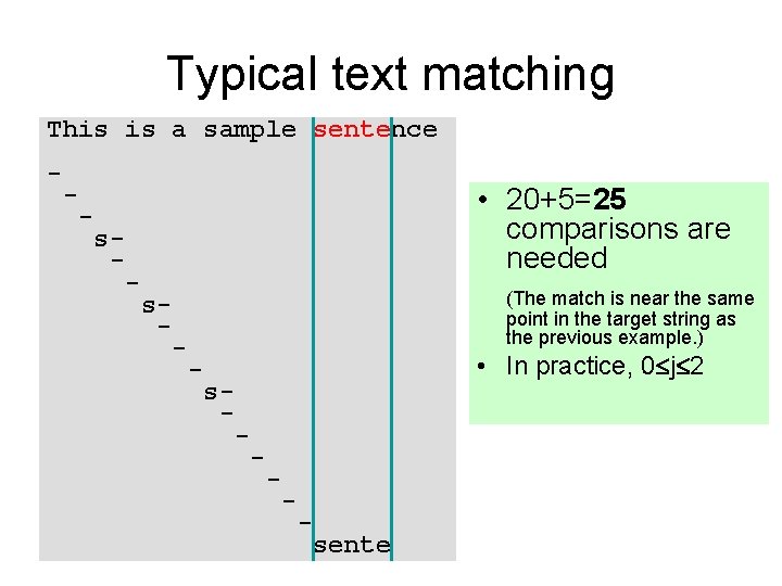
Typical text matching This is a sample sentence - - • 20+5=25 comparisons are needed - s- - (The match is near the same point in the target string as the previous example. ) s- - • In practice, 0 j 2 - s- - - sente

String Matching • Brute force worst case – O(MN) – Expensive for long patterns in repetitive text • How to improve on this? • Intuition: – Remember what is learned from previous matches

Finite State Machines

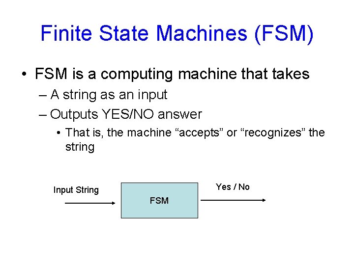
Finite State Machines (FSM) • FSM is a computing machine that takes – A string as an input – Outputs YES/NO answer • That is, the machine “accepts” or “recognizes” the string Yes / No Input String FSM

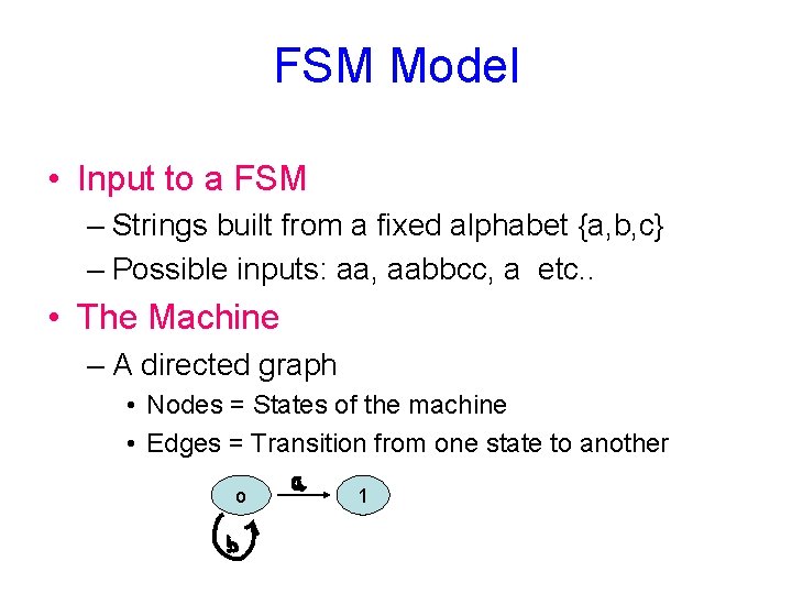
FSM Model • Input to a FSM – Strings built from a fixed alphabet {a, b, c} – Possible inputs: aa, aabbcc, a etc. . • The Machine – A directed graph • Nodes = States of the machine • Edges = Transition from one state to another o 1

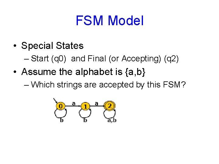
FSM Model • Special States – Start (q 0) and Final (or Accepting) (q 2) • Assume the alphabet is {a, b} – Which strings are accepted by this FSM?

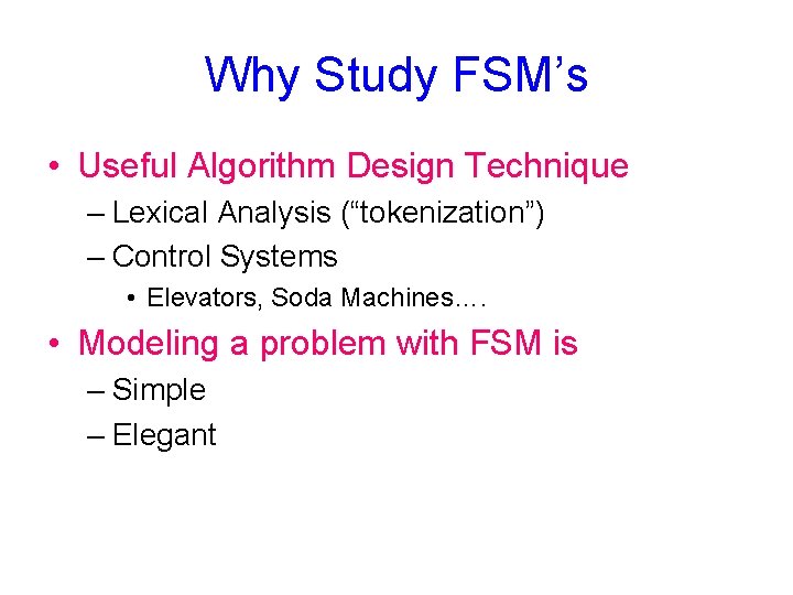
Why Study FSM’s • Useful Algorithm Design Technique – Lexical Analysis (“tokenization”) – Control Systems • Elevators, Soda Machines…. • Modeling a problem with FSM is – Simple – Elegant

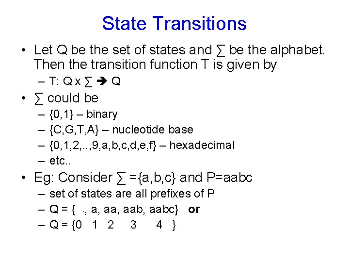
State Transitions • Let Q be the set of states and ∑ be the alphabet. Then the transition function T is given by – T: Q x ∑ Q • ∑ could be – – {0, 1} – binary {C, G, T, A} – nucleotide base {0, 1, 2, . . , 9, a, b, c, d, e, f} – hexadecimal etc. . • Eg: Consider ∑ ={a, b, c} and P=aabc – set of states are all prefixes of P – Q = {Ǿ, a, aab, aabc} or – Q = {0 1 2 3 4 }

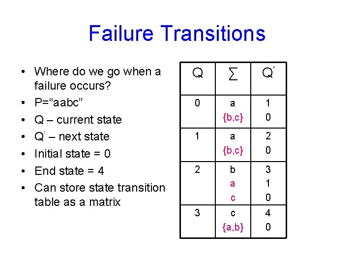
Failure Transitions • Where do we go when a failure occurs? • P=“aabc” • Q – current state • Q’ – next state • Initial state = 0 • End state = 4 • Can store state transition table as a matrix Q ∑ Q’ 0 a {b, c} 1 0 1 a {b, c} 2 0 2 b a c 3 1 0 3 c {a, b} 4 0

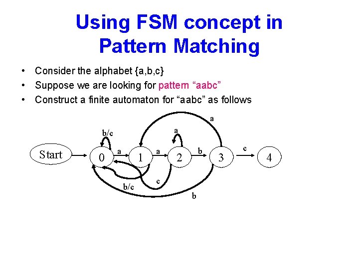
Using FSM concept in Pattern Matching • Consider the alphabet {a, b, c} • Suppose we are looking for pattern “aabc” • Construct a finite automaton for “aabc” as follows a a b/c Start 0 a 1 b/c a b 2 c b 3 c 4

Knuth Morris Pratt (KMP) Algorithm

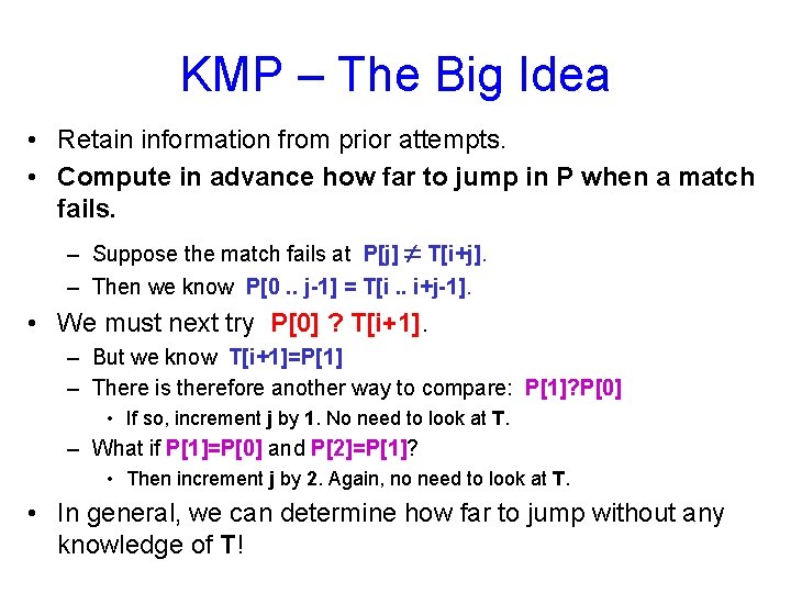
KMP – The Big Idea • Retain information from prior attempts. • Compute in advance how far to jump in P when a match fails. – Suppose the match fails at P[j] T[i+j]. – Then we know P[0. . j-1] = T[i. . i+j-1]. • We must next try P[0] ? T[i+1]. – But we know T[i+1]=P[1] – There is therefore another way to compare: P[1]? P[0] • If so, increment j by 1. No need to look at T. – What if P[1]=P[0] and P[2]=P[1]? • Then increment j by 2. Again, no need to look at T. • In general, we can determine how far to jump without any knowledge of T!

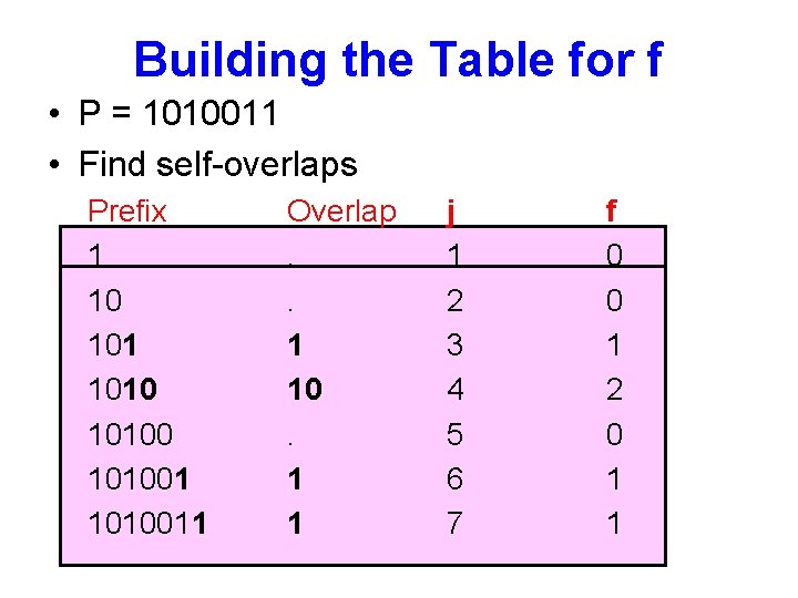
Implementing KMP • Never decrement i, ever. – Comparing T[i] with P[j]. • Compute a table f of how far to jump j forward when a match fails. – The next match will compare T[i] with P[f[j-1]] • Do this by matching P against itself in all positions.

Building the Table for f • P = 1010011 • Find self-overlaps Prefix 1 10 101001 1010011 Overlap. . 1 10. 1 1 j 1 2 3 4 5 6 7 f 0 0 1 2 0 1 1

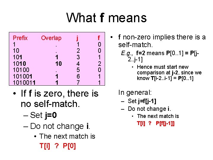
What f means Prefix Overlap 1. 101 1 1010 10 101001 1 1010011 1 j 1 2 3 4 5 6 7 f 0 0 1 2 0 1 1 • If f is zero, there is no self-match. – Set j=0 – Do not change i. • The next match is T[i] ? P[0] • f non-zero implies there is a self-match. E. g. , f=2 means P[0. . 1] = P[j 2. . j-1] • Hence must start new comparison at j-2, since we know T[i-2. . i-1] = P[0. . 1] In general: – Set j=f[j-1] – Do not change i. • The next match is T[i] ? P[f[j-1]]

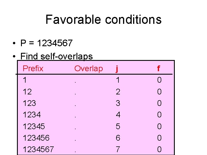
Favorable conditions • P = 1234567 • Find self-overlaps Prefix 1 12 123456 1234567 Overlap. . . . j 1 2 3 4 5 6 7 f 0 0 0 0

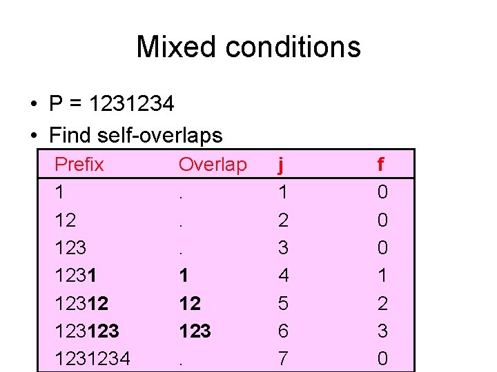
Mixed conditions • P = 1231234 • Find self-overlaps Prefix 1 12 123123 1231234 Overlap. . . 1 12 123. j 1 2 3 4 5 6 7 f 0 0 0 1 2 3 0

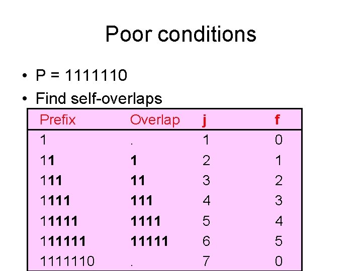
Poor conditions • P = 1111110 • Find self-overlaps Prefix 1 11 111111 1111110 Overlap. 1 11 11111. j 1 2 3 4 5 6 7 f 0 1 2 3 4 5 0

KMP pre-process Algorithm m = |P|; Define a table F of size m F[0] = 0; i = 1; j = 0; while(i<m) { compare P[i] and P[j]; if(P[j]==P[i]) { F[i] = j+1; i++; j++; } else if (j>0) j=F[j-1]; else {F[i] = 0; i++; } } Use previous values of f

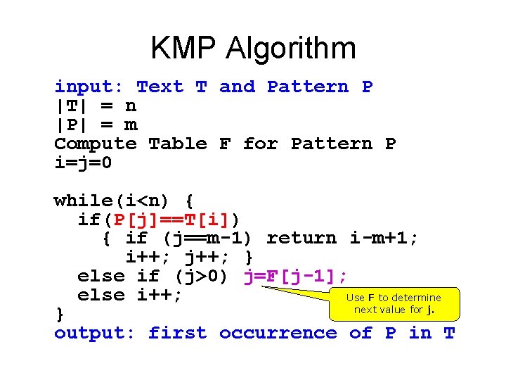
KMP Algorithm input: Text T and Pattern P |T| = n |P| = m Compute Table F for Pattern P i=j=0 while(i<n) { if(P[j]==T[i]) { if (j==m-1) return i-m+1; i++; j++; } else if (j>0) j=F[j-1]; else i++; Use F to determine next value for j. } output: first occurrence of P in T

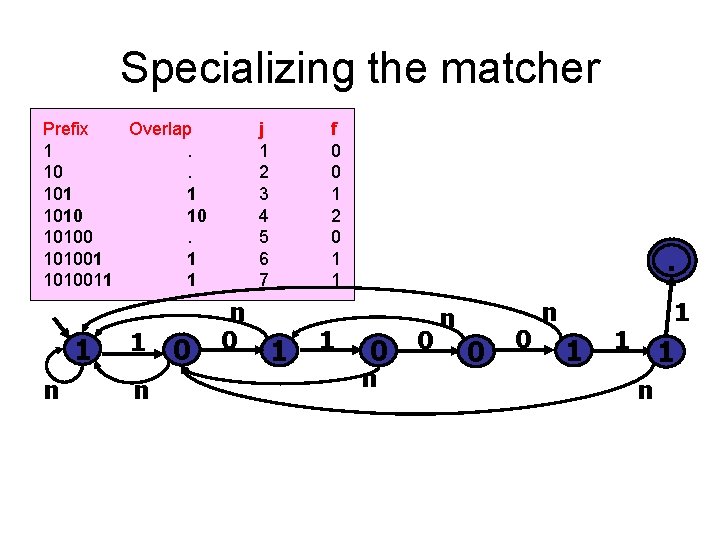
Specializing the matcher Prefix Overlap 1. 101 1 1010 10 101001 1 1010011 1 1 n 0 j 1 2 3 4 5 6 7 n 0 f 0 0 1 2 0 1 1 . 0 0 n 1 1 n

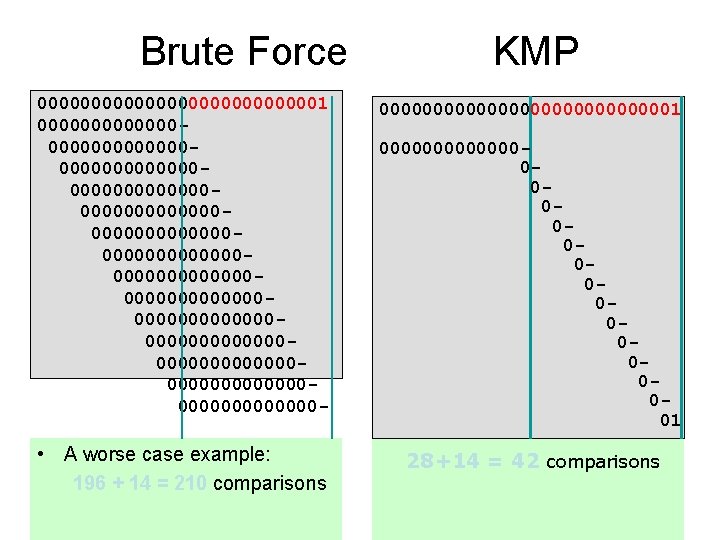
Brute Force KMP 00000000000001 0000000000000000000000000000000000000000000000000000000000000000000000000000000000000000000 - 000000000000001 • A worse case example: 196 + 14 = 210 comparisons 28+14 = 42 comparisons 000000000000001

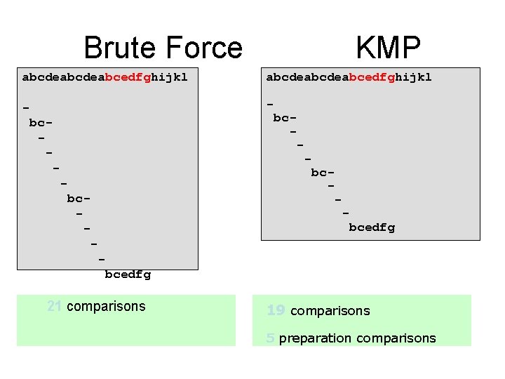
Brute Force KMP abcdeabcdeabcedfghijkl - bc- bc- - bcedfg 21 comparisons 19 comparisons 5 preparation comparisons

KMP Performance • At each iteration, one of three cases: – T[i] = P[j] • i increases – T[i] <> P[j] and j>0 • i-j increases – T[I] <> P[j] and j=0 • i increases and i-j increases • Hence, maximum of 2 N iterations. • Constructing f[] needs 2 M iterations. • Thus worst case performance is O(N+M).

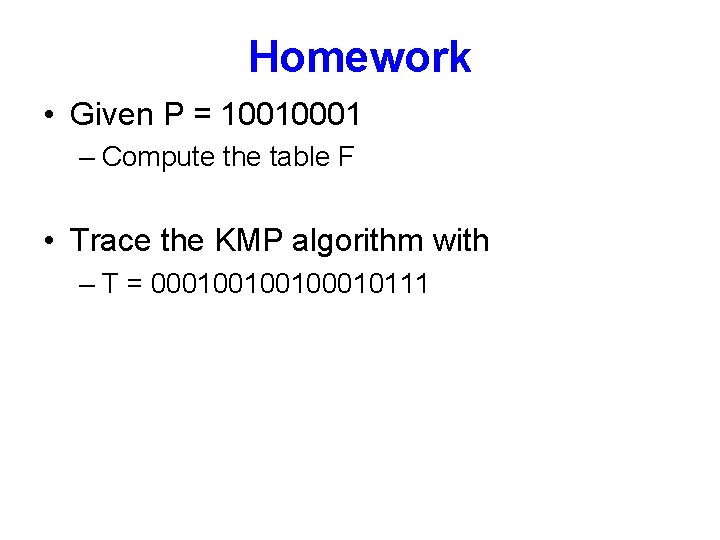
Homework • Given P = 10010001 – Compute the table F • Trace the KMP algorithm with – T = 00010010010111