Genome Evolution Amos Tanay The Weizmann Institute Genome

Genome Evolution © Amos Tanay, The Weizmann Institute Genome evolution Lecture 2: population genetics I: drift and mutation

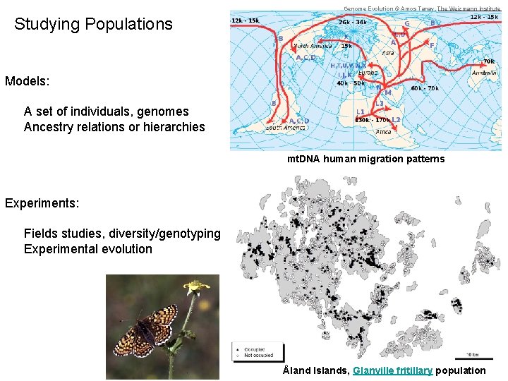
Genome Evolution © Amos Tanay, The Weizmann Institute Studying Populations Models: A set of individuals, genomes Ancestry relations or hierarchies mt. DNA human migration patterns Experiments: Fields studies, diversity/genotyping Experimental evolution Åland Islands, Glanville fritillary population

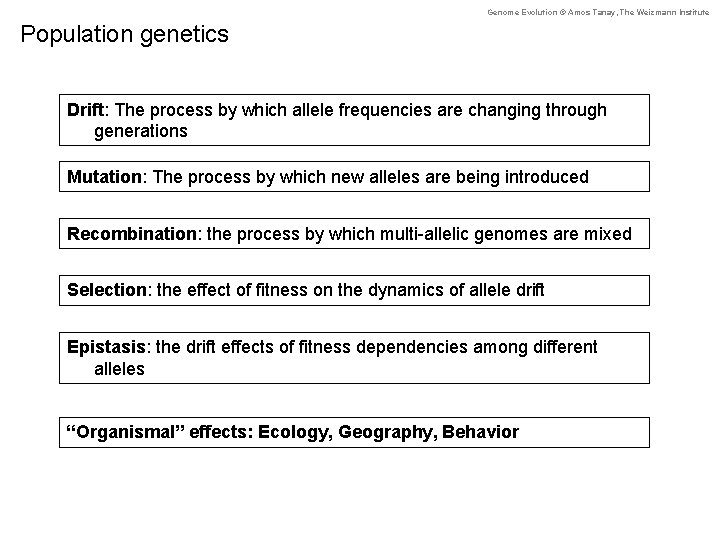
Genome Evolution © Amos Tanay, The Weizmann Institute Population genetics Drift: The process by which allele frequencies are changing through generations Mutation: The process by which new alleles are being introduced Recombination: the process by which multi-allelic genomes are mixed Selection: the effect of fitness on the dynamics of allele drift Epistasis: the drift effects of fitness dependencies among different alleles “Organismal” effects: Ecology, Geography, Behavior

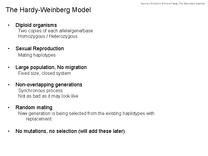
Genome Evolution © Amos Tanay, The Weizmann Institute The Hardy-Weinberg Model • Diploid organisms Two copies of each allele/gene/base Homozygous / Heterozygous • Sexual Reproduction Mating haplotypes • Large population, No migration Fixed size, closed system • Non-overlapping generations Synchronous process Not as bad as it may look like • Random mating New generation is being selected from the existing haplotypes with replacement • No mutations, no selection (will add these later)

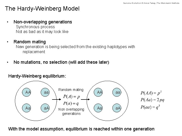
Genome Evolution © Amos Tanay, The Weizmann Institute The Hardy-Weinberg Model • Non-overlapping generations Synchronous process Not as bad as it may look like • Random mating New generation is being selected from the existing haplotypes with replacement • No mutations, no selection (will add these later) Hardy-Weinberg equilibrium: AA aa Aa a. A Random mating Non overlapping generations AA aa Aa a. A With the model assumption, equilibrium is reached within one generation

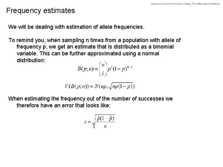
Genome Evolution © Amos Tanay, The Weizmann Institute Frequency estimates We will be dealing with estimation of allele frequencies. To remind you, when sampling n times from a population with allele of frequency p, we get an estimate that is distributed as a binomial variable. This can be further approximated using a normal distribution: When estimating the frequency out of the number of successes we therefore have an error that looks like:

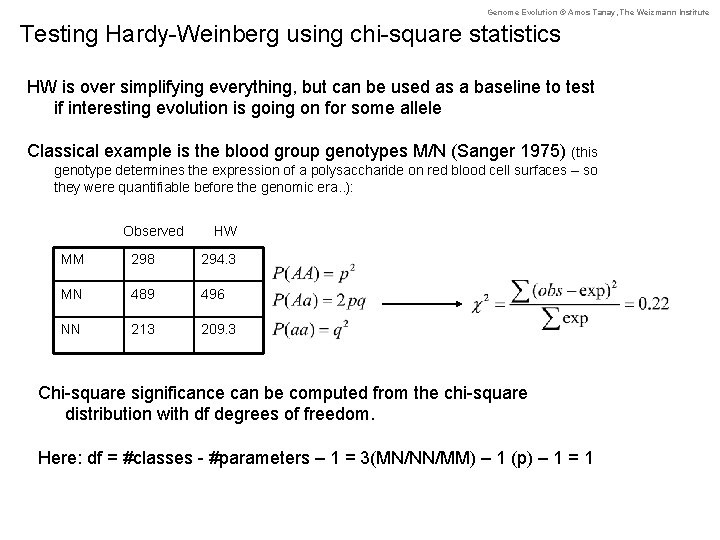
Genome Evolution © Amos Tanay, The Weizmann Institute Testing Hardy-Weinberg using chi-square statistics HW is over simplifying everything, but can be used as a baseline to test if interesting evolution is going on for some allele Classical example is the blood group genotypes M/N (Sanger 1975) (this genotype determines the expression of a polysaccharide on red blood cell surfaces – so they were quantifiable before the genomic era. . ): Observed HW MM 298 294. 3 MN 489 496 NN 213 209. 3 Chi-square significance can be computed from the chi-square distribution with df degrees of freedom. Here: df = #classes - #parameters – 1 = 3(MN/NN/MM) – 1 (p) – 1 = 1

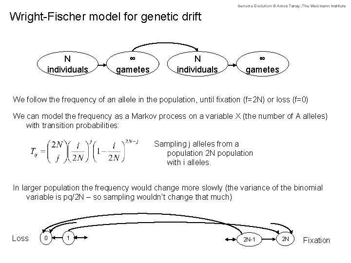
Genome Evolution © Amos Tanay, The Weizmann Institute Wright-Fischer model for genetic drift N individuals ∞ gametes We follow the frequency of an allele in the population, until fixation (f=2 N) or loss (f=0) We can model the frequency as a Markov process on a variable X (the number of A alleles) with transition probabilities: Sampling j alleles from a population 2 N population with i alleles. In larger population the frequency would change more slowly (the variance of the binomial variable is pq/2 N – so sampling wouldn’t change that much) Loss 0 1 2 N-1 2 N Fixation

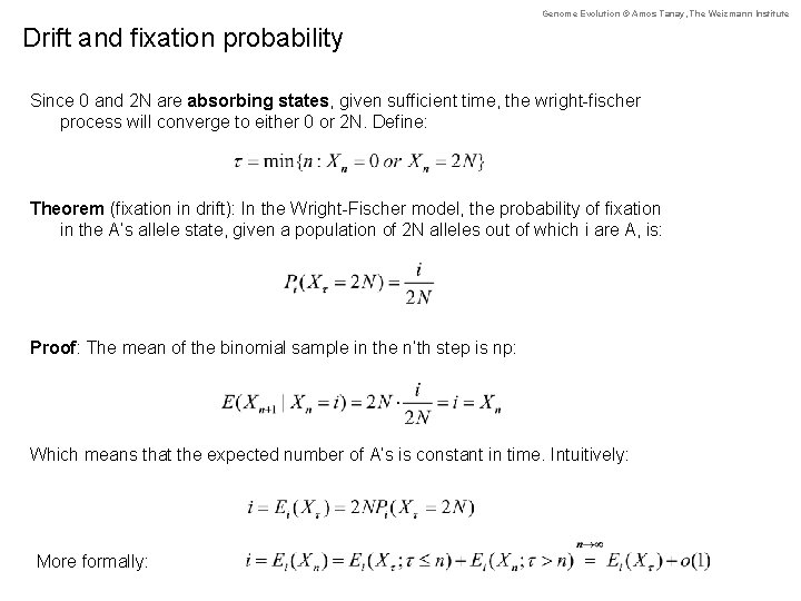
Genome Evolution © Amos Tanay, The Weizmann Institute Drift and fixation probability Since 0 and 2 N are absorbing states, given sufficient time, the wright-fischer process will converge to either 0 or 2 N. Define: Theorem (fixation in drift): In the Wright-Fischer model, the probability of fixation in the A’s allele state, given a population of 2 N alleles out of which i are A, is: Proof: The mean of the binomial sample in the n’th step is np: Which means that the expected number of A’s is constant in time. Intuitively: More formally:

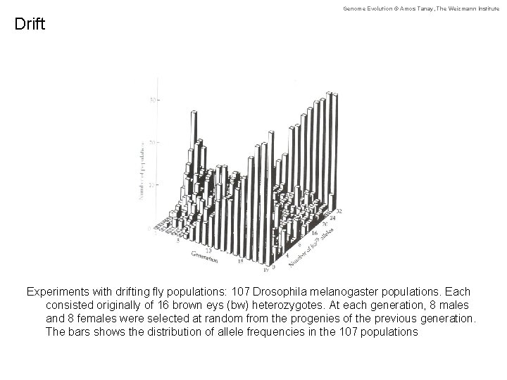
Genome Evolution © Amos Tanay, The Weizmann Institute Drift Figure 7. 4 Experiments with drifting fly populations: 107 Drosophila melanogaster populations. Each consisted originally of 16 brown eys (bw) heterozygotes. At each generation, 8 males and 8 females were selected at random from the progenies of the previous generation. The bars shows the distribution of allele frequencies in the 107 populations

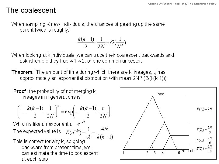
Genome Evolution © Amos Tanay, The Weizmann Institute The coalescent When sampling K new individuals, the chances of peaking up the same parent twice is roughly: When looking at k individuals, we can trace their coalescent backwards and ask when did they had k-1, k-2, or one common ancestor. Theorem: The amount of time during which there are k lineages, tk has approximately an exponential distribution with mean 2 N * (2/(k(k-1))) Proof: the probability of not merging k lineages in n generations is: Past Which is like an exponential The expected value is This is correct for any k, so going backward from present time, we can estimate the time to coalescent at each step 1 2 3 4 5 Present

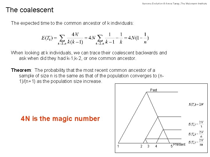
Genome Evolution © Amos Tanay, The Weizmann Institute The coalescent The expected time to the common ancestor of k individuals: When looking at k individuals, we can trace their coalescent backwards and ask when did they had k-1, k-2, or one common ancestor. Theorem: The probability that the most recent common ancestor of a sample of size n is the same as that of the population converges to (n 1)/(n+1) as the population size increase. Past 4 N is the magic number 1 2 3 4 5 Present

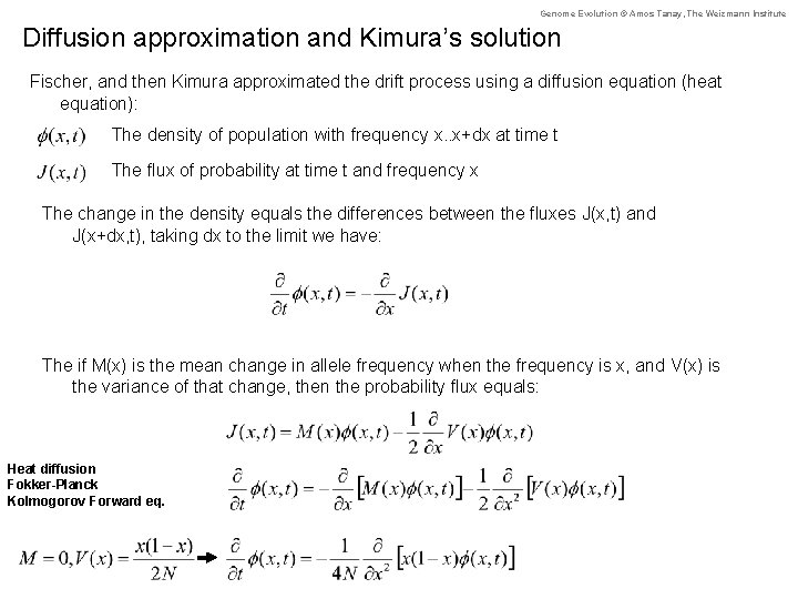
Genome Evolution © Amos Tanay, The Weizmann Institute Diffusion approximation and Kimura’s solution Fischer, and then Kimura approximated the drift process using a diffusion equation (heat equation): The density of population with frequency x. . x+dx at time t The flux of probability at time t and frequency x The change in the density equals the differences between the fluxes J(x, t) and J(x+dx, t), taking dx to the limit we have: The if M(x) is the mean change in allele frequency when the frequency is x, and V(x) is the variance of that change, then the probability flux equals: Heat diffusion Fokker-Planck Kolmogorov Forward eq.

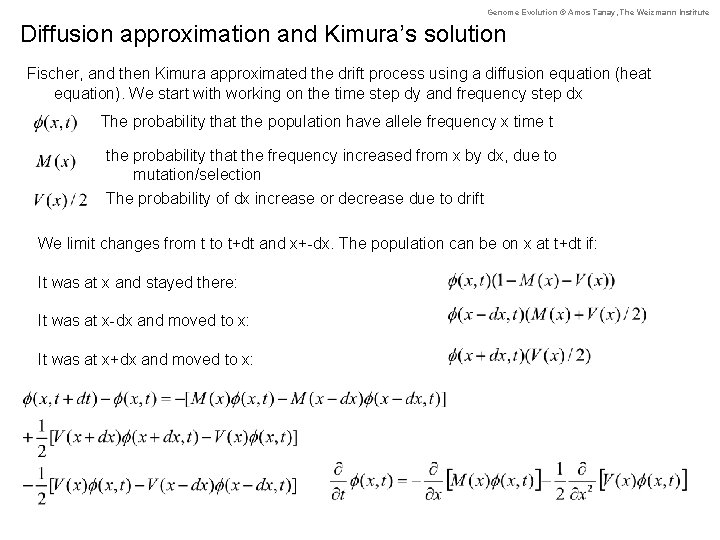
Genome Evolution © Amos Tanay, The Weizmann Institute Diffusion approximation and Kimura’s solution Fischer, and then Kimura approximated the drift process using a diffusion equation (heat equation). We start with working on the time step dy and frequency step dx The probability that the population have allele frequency x time t the probability that the frequency increased from x by dx, due to mutation/selection The probability of dx increase or decrease due to drift We limit changes from t to t+dt and x+-dx. The population can be on x at t+dt if: It was at x and stayed there: It was at x-dx and moved to x: It was at x+dx and moved to x:

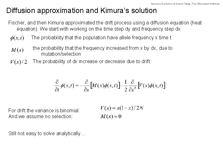
Genome Evolution © Amos Tanay, The Weizmann Institute Diffusion approximation and Kimura’s solution Fischer, and then Kimura approximated the drift process using a diffusion equation (heat equation). We start with working on the time step dy and frequency step dx The probability that the population have allele frequency x time t the probability that the frequency increased from x by dx, due to mutation/selection The probability of dx increase or decrease due to drift For drift the variance is binomial: And we assume no selection: Still not easy to solve analytically…

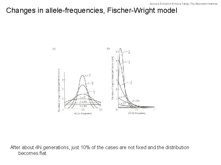
Genome Evolution © Amos Tanay, The Weizmann Institute Changes in allele-frequencies, Fischer-Wright model After about 4 N generations, just 10% of the cases are not fixed and the distribution becomes flat.

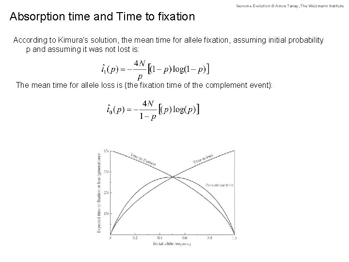
Genome Evolution © Amos Tanay, The Weizmann Institute Absorption time and Time to fixation According to Kimura’s solution, the mean time for allele fixation, assuming initial probability p and assuming it was not lost is: The mean time for allele loss is (the fixation time of the complement event):

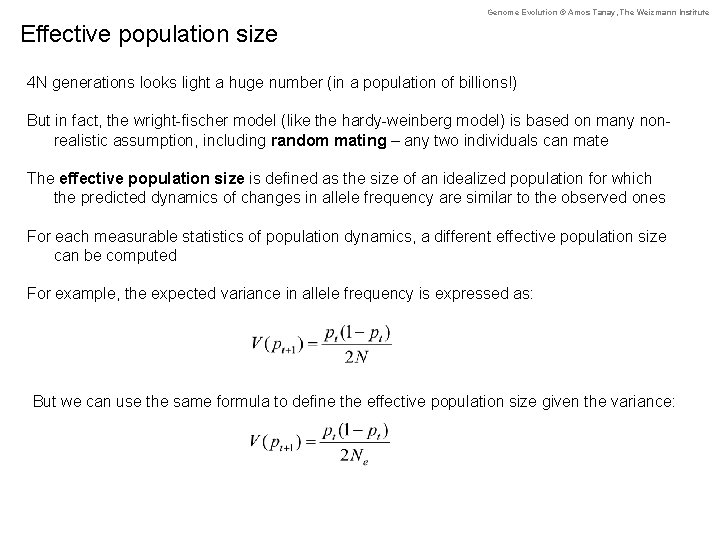
Genome Evolution © Amos Tanay, The Weizmann Institute Effective population size 4 N generations looks light a huge number (in a population of billions!) But in fact, the wright-fischer model (like the hardy-weinberg model) is based on many nonrealistic assumption, including random mating – any two individuals can mate The effective population size is defined as the size of an idealized population for which the predicted dynamics of changes in allele frequency are similar to the observed ones For each measurable statistics of population dynamics, a different effective population size can be computed For example, the expected variance in allele frequency is expressed as: But we can use the same formula to define the effective population size given the variance:

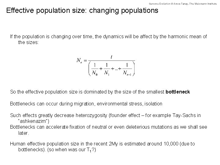
Genome Evolution © Amos Tanay, The Weizmann Institute Effective population size: changing populations If the population is changing over time, the dynamics will be affect by the harmonic mean of the sizes: So the effective population size is dominated by the size of the smallest bottleneck Bottlenecks can occur during migration, environmental stress, isolation Such effects greatly decrease heterozygosity (founder effect – for example Tay-Sachs in “ashkenazim”) Bottlenecks can accelerate fixation of neutral or even deleterious mutations as we shall see later. Human effective population size in the recent 2 My is estimated around 10, 000 (due to bottlenecks). (so when was our T 1? )

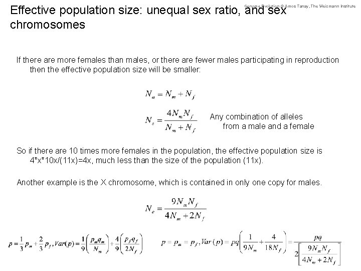
Effective population size: unequal sex ratio, and sex chromosomes Genome Evolution © Amos Tanay, The Weizmann Institute If there are more females than males, or there are fewer males participating in reproduction the effective population size will be smaller: Any combination of alleles from a male and a female So if there are 10 times more females in the population, the effective population size is 4*x*10 x/(11 x)=4 x, much less than the size of the population (11 x). Another example is the X chromosome, which is contained in only one copy for males.

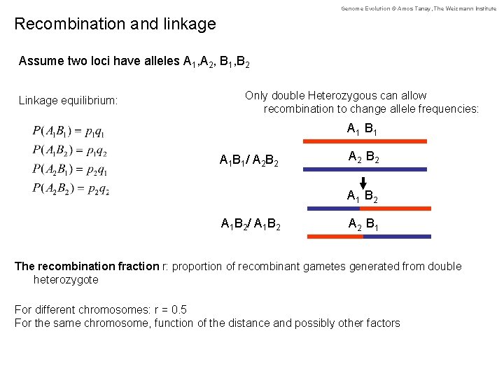
Genome Evolution © Amos Tanay, The Weizmann Institute Recombination and linkage Assume two loci have alleles A 1, A 2, B 1, B 2 Linkage equilibrium: Only double Heterozygous can allow recombination to change allele frequencies: A 1 B 1 A 1 B 1/ A 2 B 2 A 2 B 2 A 1 B 2/ A 1 B 2 A 2 B 1 The recombination fraction r: proportion of recombinant gametes generated from double heterozygote For different chromosomes: r = 0. 5 For the same chromosome, function of the distance and possibly other factors

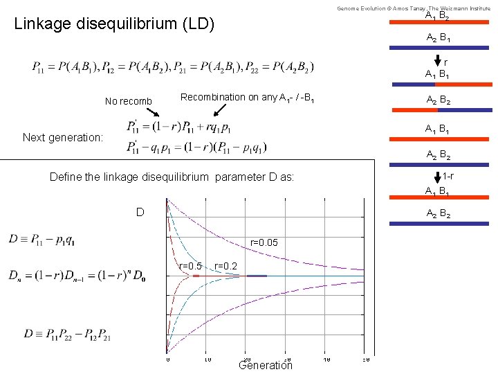
Genome Evolution © Amos Tanay, The Weizmann Institute A 1 B 2 Linkage disequilibrium (LD) A 2 B 1 r A 1 B 1 No recomb Recombination on any A 1 - / -B 1 A 2 B 2 A 1 B 1 Next generation: A 2 B 2 Define the linkage disequilibrium parameter D as: 1 -r A 1 B 1 D A 2 B 2 r=0. 05 r=0. 2 Generation

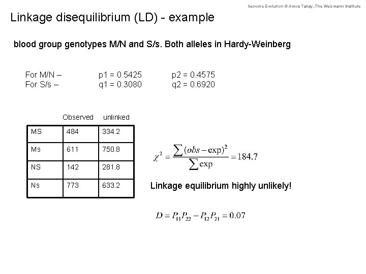
Genome Evolution © Amos Tanay, The Weizmann Institute Linkage disequilibrium (LD) - example blood group genotypes M/N and S/s. Both alleles in Hardy-Weinberg For M/N – For S/s – p 1 = 0. 5425 q 1 = 0. 3080 Observed p 2 = 0. 4575 q 2 = 0. 6920 unlinked MS 484 334. 2 Ms 611 750. 8 NS 142 281. 8 Ns 773 633. 2 Linkage equilibrium highly unlikely!

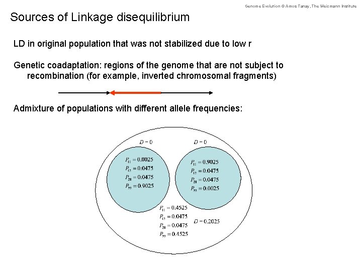
Genome Evolution © Amos Tanay, The Weizmann Institute Sources of Linkage disequilibrium LD in original population that was not stabilized due to low r Genetic coadaptation: regions of the genome that are not subject to recombination (for example, inverted chromosomal fragments) Admixture of populations with different allele frequencies:

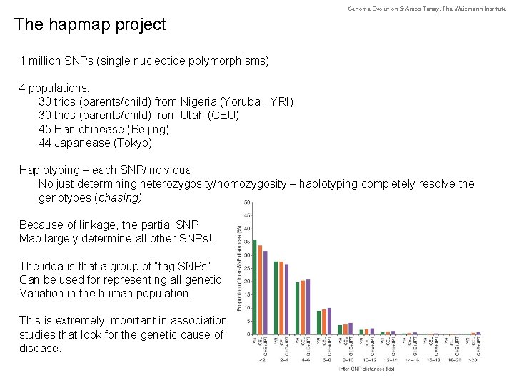
Genome Evolution © Amos Tanay, The Weizmann Institute The hapmap project 1 million SNPs (single nucleotide polymorphisms) 4 populations: 30 trios (parents/child) from Nigeria (Yoruba - YRI) 30 trios (parents/child) from Utah (CEU) 45 Han chinease (Beijing) 44 Japanease (Tokyo) Haplotyping – each SNP/individual No just determining heterozygosity/homozygosity – haplotyping completely resolve the genotypes (phasing) Because of linkage, the partial SNP Map largely determine all other SNPs!! The idea is that a group of “tag SNPs” Can be used for representing all genetic Variation in the human population. This is extremely important in association studies that look for the genetic cause of disease.

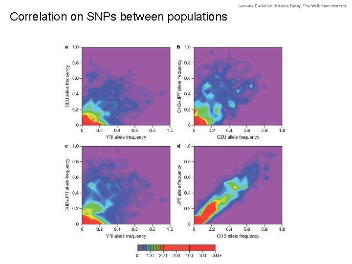
Genome Evolution © Amos Tanay, The Weizmann Institute Correlation on SNPs between populations

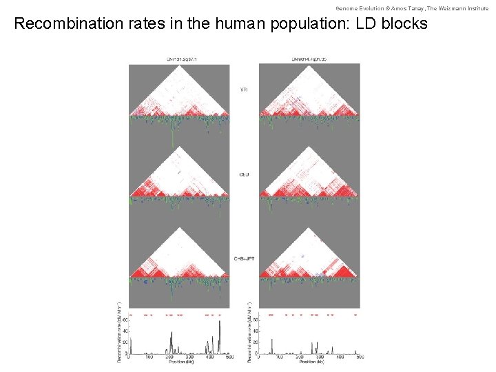
Genome Evolution © Amos Tanay, The Weizmann Institute Recombination rates in the human population: LD blocks

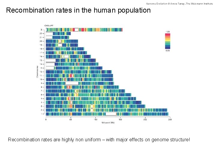
Genome Evolution © Amos Tanay, The Weizmann Institute Recombination rates in the human population Recombination rates are highly non uniform – with major effects on genome structure!

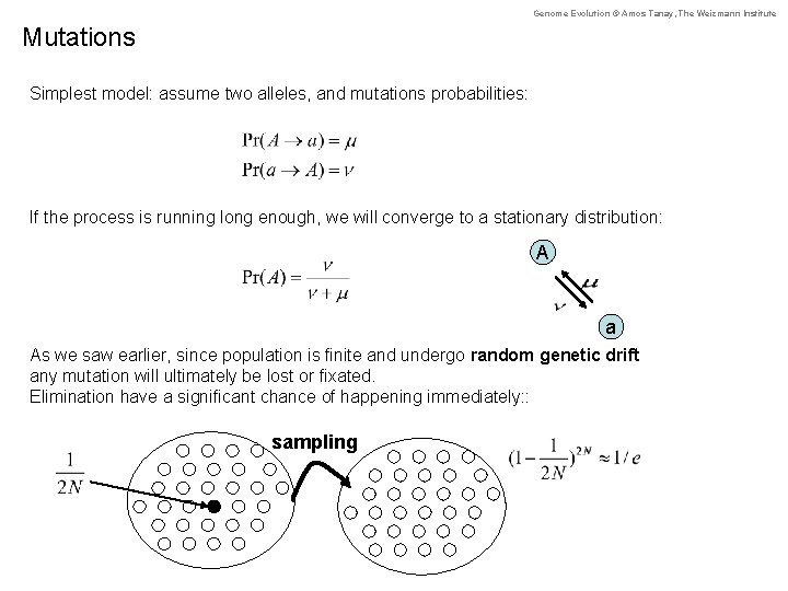
Genome Evolution © Amos Tanay, The Weizmann Institute Mutations Simplest model: assume two alleles, and mutations probabilities: If the process is running long enough, we will converge to a stationary distribution: A a As we saw earlier, since population is finite and undergo random genetic drift any mutation will ultimately be lost or fixated. Elimination have a significant chance of happening immediately: : sampling

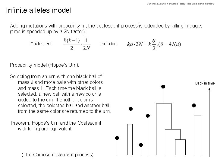
Genome Evolution © Amos Tanay, The Weizmann Institute Infinite alleles model Adding mutations with probability m, the coalescent process is extended by killing lineages (time is speeded up by a 2 N factor): Coalescent: mutation: Probability model (Hoppe’s Urn): Selecting from an urn with one black ball of mass q and more balls with other colors and mass 1. Each time the black ball is selected, a new ball with a new color is added to the urn. If another color is selected, the selected ball and another ball from the same color are returned to the urn. Theorem: Hoppe’s Urn and the Coalescent with killing are equivalent (The Chinese restaurant process) Back in time

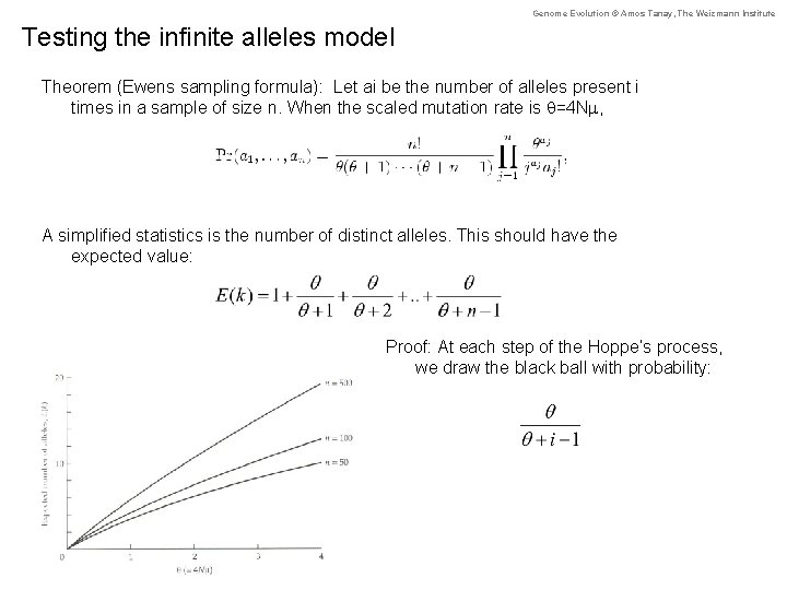
Genome Evolution © Amos Tanay, The Weizmann Institute Testing the infinite alleles model Theorem (Ewens sampling formula): Let ai be the number of alleles present i times in a sample of size n. When the scaled mutation rate is q=4 Nm, A simplified statistics is the number of distinct alleles. This should have the expected value: Proof: At each step of the Hoppe’s process, we draw the black ball with probability:

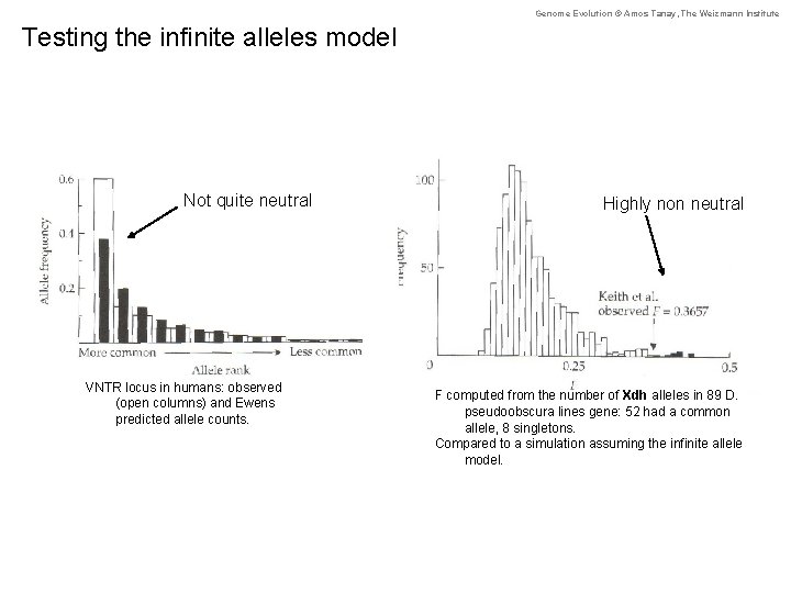
Genome Evolution © Amos Tanay, The Weizmann Institute Testing the infinite alleles model Figure 7. 16, 7. 17 Not quite neutral VNTR locus in humans: observed (open columns) and Ewens predicted allele counts. Highly non neutral F computed from the number of Xdh alleles in 89 D. pseudoobscura lines gene: 52 had a common allele, 8 singletons. Compared to a simulation assuming the infinite allele model.