Genome Evolution Amos Tanay 2009 Genome evolution Lecture

Genome Evolution. Amos Tanay 2009 Genome evolution Lecture 3: population genetics II: selection

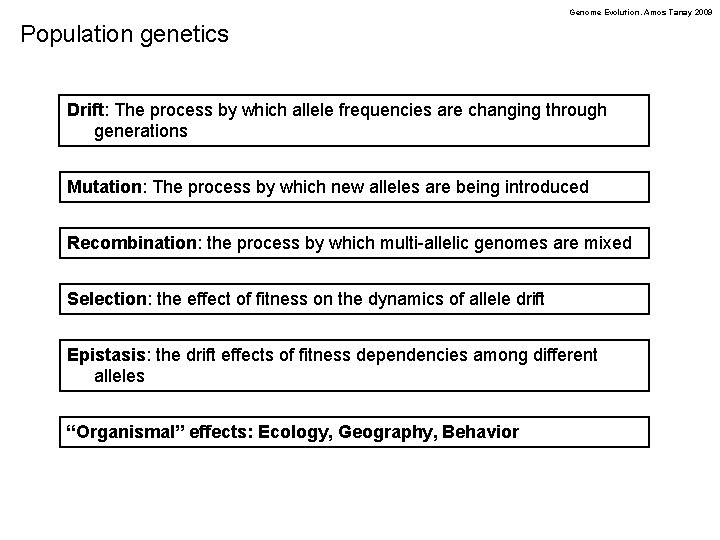
Genome Evolution. Amos Tanay 2009 Population genetics Drift: The process by which allele frequencies are changing through generations Mutation: The process by which new alleles are being introduced Recombination: the process by which multi-allelic genomes are mixed Selection: the effect of fitness on the dynamics of allele drift Epistasis: the drift effects of fitness dependencies among different alleles “Organismal” effects: Ecology, Geography, Behavior

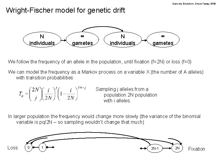
Genome Evolution. Amos Tanay 2009 Wright-Fischer model for genetic drift N individuals ∞ gametes We follow the frequency of an allele in the population, until fixation (f=2 N) or loss (f=0) We can model the frequency as a Markov process on a variable X (the number of A alleles) with transition probabilities: Sampling j alleles from a population 2 N population with i alleles. In larger population the frequency would change more slowly (the variance of the binomial variable is pq/2 N – so sampling wouldn’t change that much) Loss 0 1 2 N-1 2 N Fixation

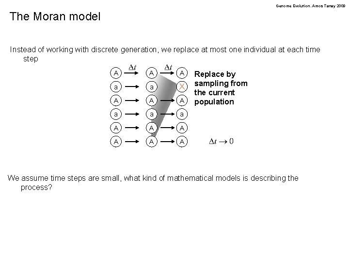
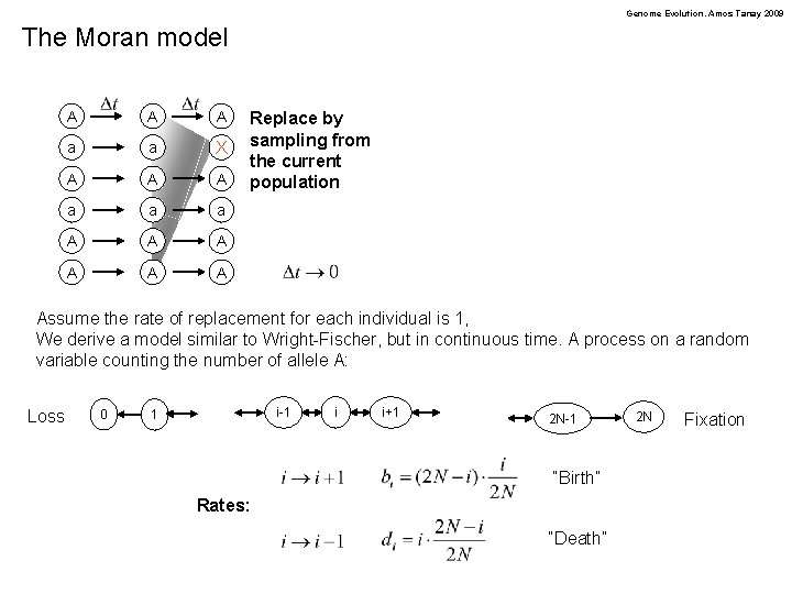
Genome Evolution. Amos Tanay 2009 The Moran model Instead of working with discrete generation, we replace at most one individual at each time step A A A a a X A A A a a a A A A Replace by sampling from the current population We assume time steps are small, what kind of mathematical models is describing the process?

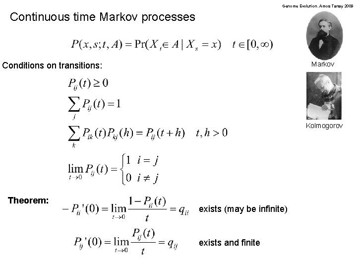
Genome Evolution. Amos Tanay 2009 Continuous time Markov processes Markov Conditions on transitions: Kolmogorov Theorem: exists (may be infinite) exists and finite

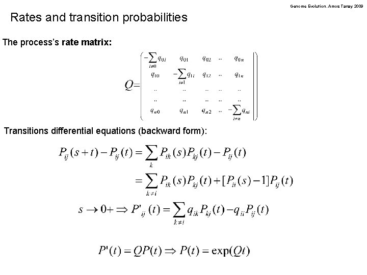
Genome Evolution. Amos Tanay 2009 Rates and transition probabilities The process’s rate matrix: Transitions differential equations (backward form):

Genome Evolution. Amos Tanay 2009 The Moran model A A A a a X A A A a a a A A A Replace by sampling from the current population Assume the rate of replacement for each individual is 1, We derive a model similar to Wright-Fischer, but in continuous time. A process on a random variable counting the number of allele A: Loss 0 i-1 1 i i+1 2 N-1 “Birth” Rates: “Death” 2 N Fixation

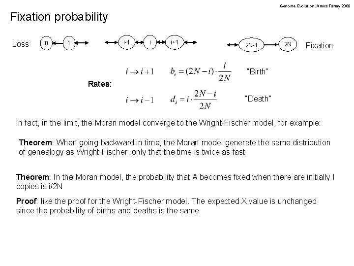
Genome Evolution. Amos Tanay 2009 Fixation probability Loss 0 i-1 1 i i+1 2 N-1 2 N Fixation “Birth” Rates: “Death” In fact, in the limit, the Moran model converge to the Wright-Fischer model, for example: Theorem: When going backward in time, the Moran model generate the same distribution of genealogy as Wright-Fischer, only that the time is twice as fast Theorem: In the Moran model, the probability that A becomes fixed when there are initially I copies is i/2 N Proof: like the proof for the Wright-Fischer model. The expected X value is unchanged since the probability of births and deaths is the same

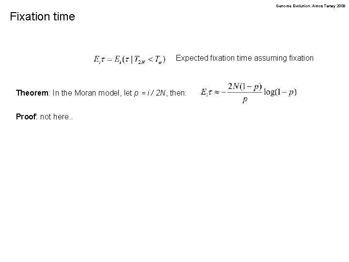
Genome Evolution. Amos Tanay 2009 Fixation time Expected fixation time assuming fixation Theorem: In the Moran model, let p = i / 2 N, then: Proof: not here. .

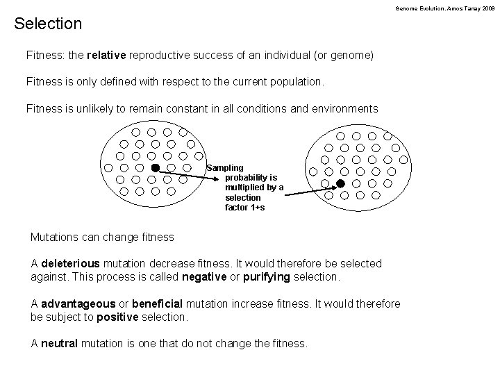
Genome Evolution. Amos Tanay 2009 Selection Fitness: the relative reproductive success of an individual (or genome) Fitness is only defined with respect to the current population. Fitness is unlikely to remain constant in all conditions and environments Sampling probability is multiplied by a selection factor 1+s Mutations can change fitness A deleterious mutation decrease fitness. It would therefore be selected against. This process is called negative or purifying selection. A advantageous or beneficial mutation increase fitness. It would therefore be subject to positive selection. A neutral mutation is one that do not change the fitness.

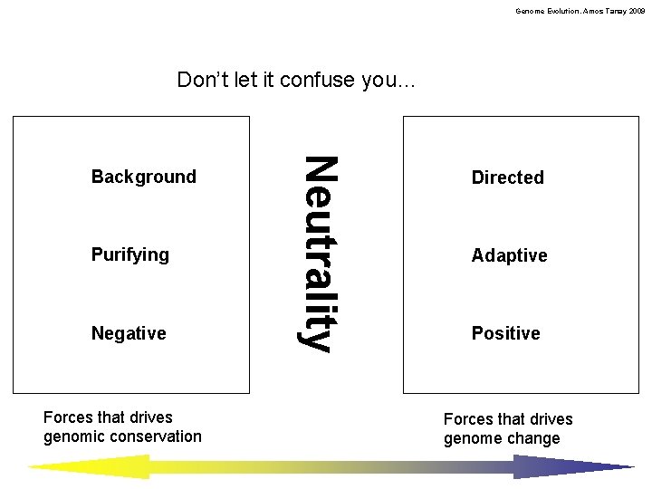
Genome Evolution. Amos Tanay 2009 Don’t let it confuse you… Purifying Negative Forces that drives genomic conservation Neutrality Background Directed Adaptive Positive Forces that drives genome change

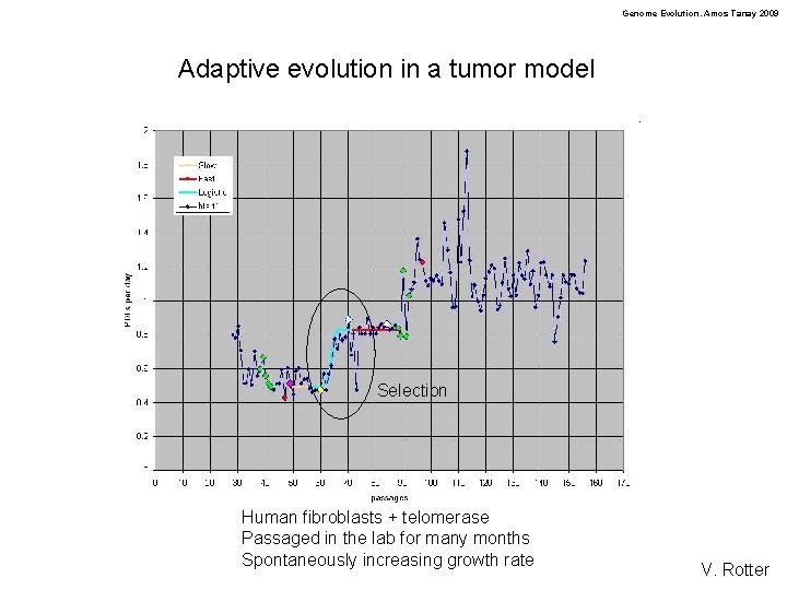
Genome Evolution. Amos Tanay 2009 Adaptive evolution in a tumor model Selection Human fibroblasts + telomerase Passaged in the lab for many months Spontaneously increasing growth rate V. Rotter

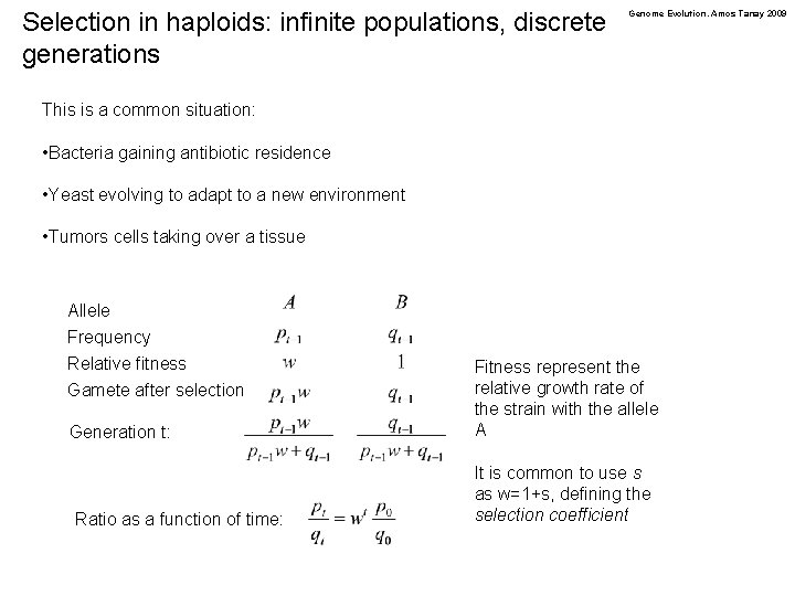
Selection in haploids: infinite populations, discrete generations Genome Evolution. Amos Tanay 2009 This is a common situation: • Bacteria gaining antibiotic residence • Yeast evolving to adapt to a new environment • Tumors cells taking over a tissue Allele Frequency Relative fitness Gamete after selection Generation t: Ratio as a function of time: Fitness represent the relative growth rate of the strain with the allele A It is common to use s as w=1+s, defining the selection coefficient

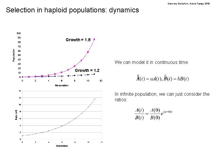
Genome Evolution. Amos Tanay 2009 Selection in haploid populations: dynamics Growth = 1. 5 We can model it in continuous time: Growth = 1. 2 In infinite population, we can just consider the ratios:

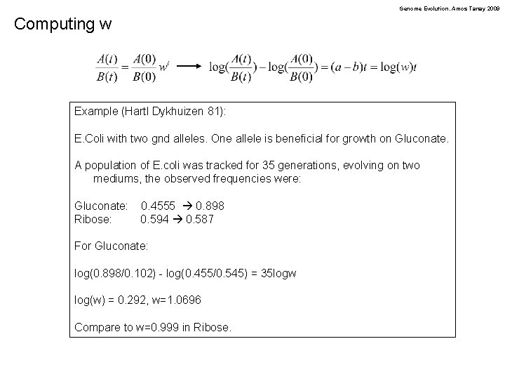
Genome Evolution. Amos Tanay 2009 Computing w Example (Hartl Dykhuizen 81): E. Coli with two gnd alleles. One allele is beneficial for growth on Gluconate. A population of E. coli was tracked for 35 generations, evolving on two mediums, the observed frequencies were: Gluconate: Ribose: 0. 4555 0. 898 0. 594 0. 587 For Gluconate: log(0. 898/0. 102) - log(0. 455/0. 545) = 35 logw log(w) = 0. 292, w=1. 0696 Compare to w=0. 999 in Ribose.

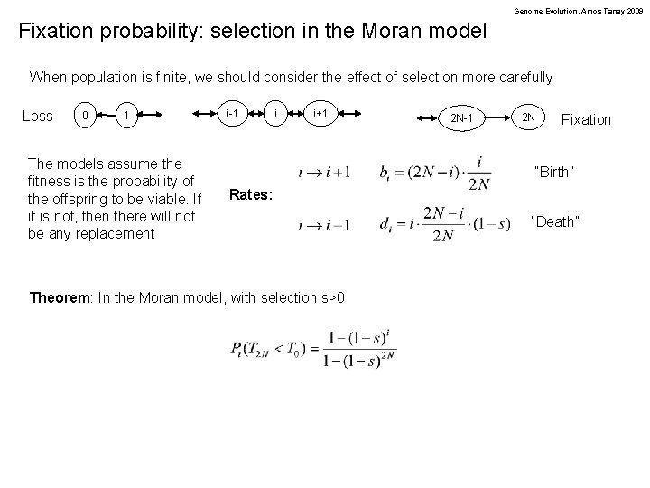
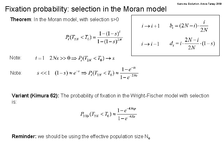
Genome Evolution. Amos Tanay 2009 Fixation probability: selection in the Moran model When population is finite, we should consider the effect of selection more carefully Loss 0 1 The models assume the fitness is the probability of the offspring to be viable. If it is not, then there will not be any replacement i-1 i i+1 2 N-1 2 N Fixation “Birth” Rates: Theorem: In the Moran model, with selection s>0 “Death”

Fixation probability: selection in the Moran model Genome Evolution. Amos Tanay 2009 Theorem: In the Moran model, with selection s>0 Note: Variant (Kimura 62): The probability of fixation in the Wright-Fischer model with selection is: Reminder: we should be using the effective population size Ne

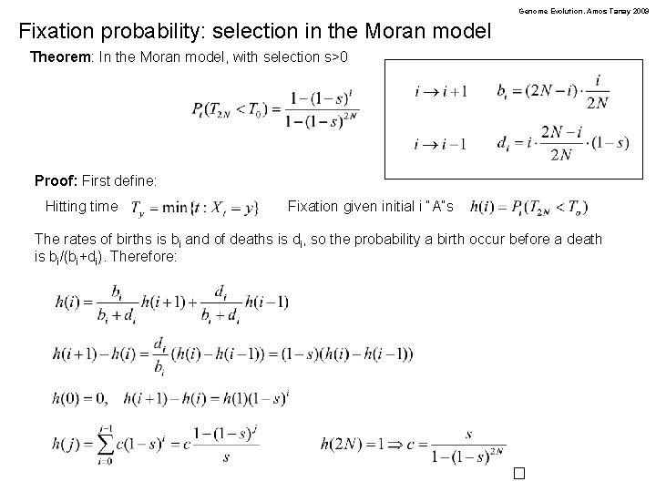
Genome Evolution. Amos Tanay 2009 Fixation probability: selection in the Moran model Theorem: In the Moran model, with selection s>0 Proof: First define: Hitting time Fixation given initial i “A”s The rates of births is bi and of deaths is di, so the probability a birth occur before a death is bi/(bi+di). Therefore:

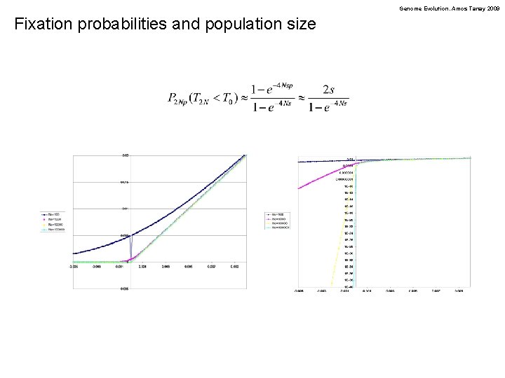
Genome Evolution. Amos Tanay 2009 Fixation probabilities and population size

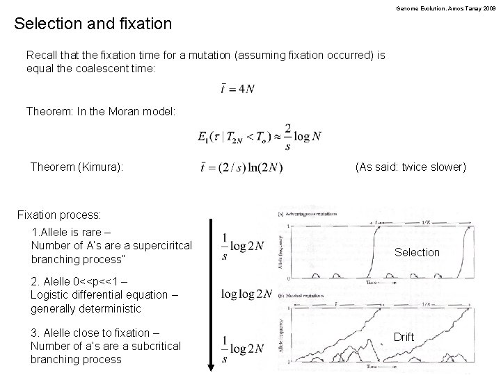
Genome Evolution. Amos Tanay 2009 Selection and fixation Recall that the fixation time for a mutation (assuming fixation occurred) is equal the coalescent time: Theorem: In the Moran model: Theorem (Kimura): (As said: twice slower) Fixation process: 1. Allele is rare – Number of A’s are a superciritcal branching process” Selection 2. Alelle 0<<p<<1 – Logistic differential equation – generally deterministic 3. Alelle close to fixation – Number of a’s are a subcritical branching process Drift

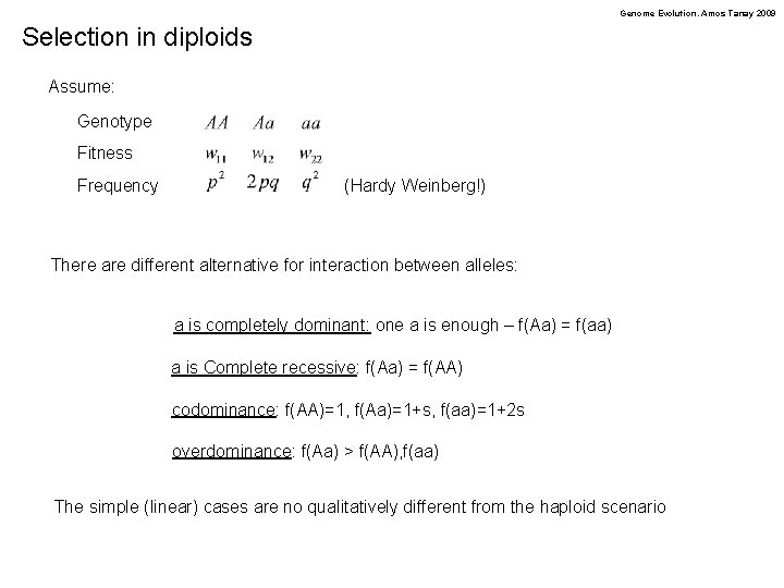
Genome Evolution. Amos Tanay 2009 Selection in diploids Assume: Genotype Fitness Frequency (Hardy Weinberg!) There are different alternative for interaction between alleles: a is completely dominant: one a is enough – f(Aa) = f(aa) a is Complete recessive: f(Aa) = f(AA) codominance: f(AA)=1, f(Aa)=1+s, f(aa)=1+2 s overdominance: f(Aa) > f(AA), f(aa) The simple (linear) cases are no qualitatively different from the haploid scenario

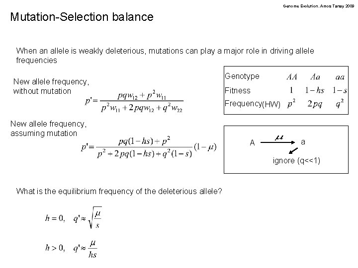
Genome Evolution. Amos Tanay 2009 Mutation-Selection balance When an allele is weakly deleterious, mutations can play a major role in driving allele frequencies New allele frequency, without mutation Genotype Fitness Frequency(HW) New allele frequency, assuming mutation A a ignore (q<<1) What is the equilibrium frequency of the deleterious allele?

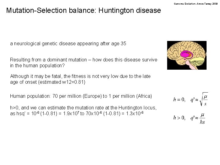
Genome Evolution. Amos Tanay 2009 Mutation-Selection balance: Huntington disease a neurological genetic disease appearing after age 35 Resulting from a dominant mutation – how does this disease survive in the human population? Although it may be fatal, the fitness is not very low due to the late age of onset (estimated w 12=0. 81) Human population: 70 per million (Europe) to 1 per million (Africa) h>0, and we can estimate the mutation rate at the Huntington locus, as hsq’ = 10 -6 (1 -0. 81) = 1. 9 x 107 to 70 x 10 -6 (1 -0. 81) = 1. 3 x 10 -6

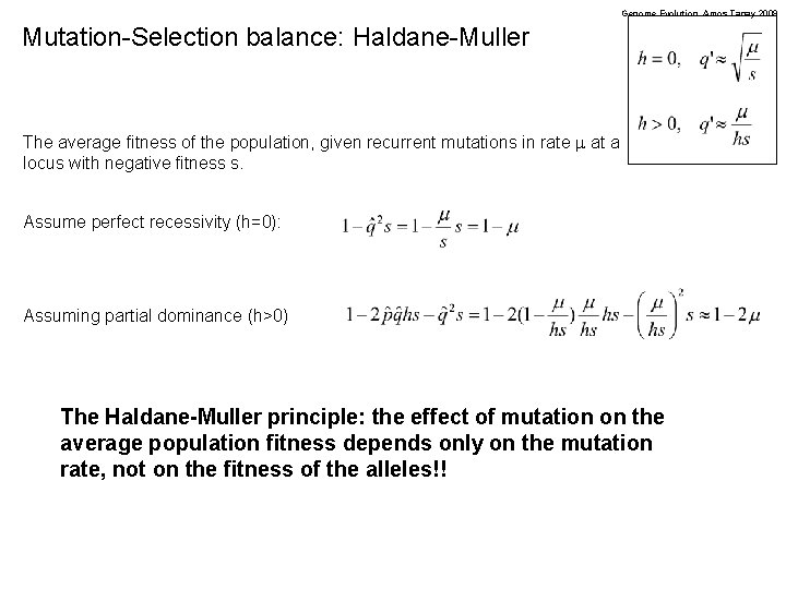
Genome Evolution. Amos Tanay 2009 Mutation-Selection balance: Haldane-Muller The average fitness of the population, given recurrent mutations in rate m at a locus with negative fitness s. Assume perfect recessivity (h=0): Assuming partial dominance (h>0) The Haldane-Muller principle: the effect of mutation on the average population fitness depends only on the mutation rate, not on the fitness of the alleles!!

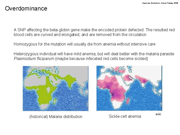
Genome Evolution. Amos Tanay 2009 Overdominance A SNP affecting the beta-globin gene make the encoded protein defected. The resulted red blood cells are curved and elongated, and are removed from the circulation Homozygous for the mutation will usually die from anemia without intensive care Heterozygous individual will have mild anemia, but will deal better with the malaria parasite Plasmodium fliciparum (maybe because infeceted red cells become sickled) (historical) Malaria distribution Sickle-cell anemia wiki

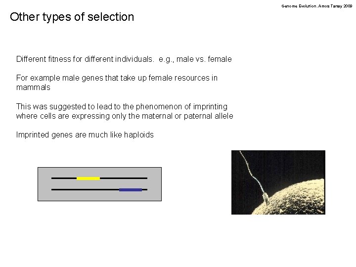
Genome Evolution. Amos Tanay 2009 Other types of selection Different fitness for different individuals. e. g. , male vs. female For example male genes that take up female resources in mammals This was suggested to lead to the phenomenon of imprinting where cells are expressing only the maternal or paternal allele Imprinted genes are much like haploids

Genome Evolution. Amos Tanay 2009 Other types of selection Frequency-, Density-dependent selection: when the fitness depend on the frequency of the allele or the population size. Fecundity selection: different reproductive potential for mating pairs. Effects of heterogeneous environment Effects that apply directly to the haplotype: gametic selection/meiotic drive (e. g. , killing your homologous chromosome reproductive potential) Sexual selection: male advertising the reproductive potential, or confronting other males Kin selection: (“origin of altruism”)

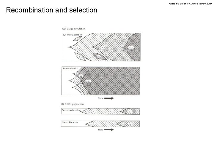
Genome Evolution. Amos Tanay 2009 Recombination and selection

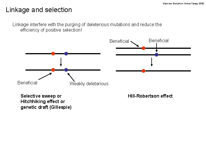
Genome Evolution. Amos Tanay 2009 Linkage and selection Linkage interfere with the purging of deleterious mutations and reduce the efficiency of positive selection! Beneficial Weakly deleterious Selective sweep or Hitchhiking effect or genetic draft (Gillespie) Hill-Robertson effect

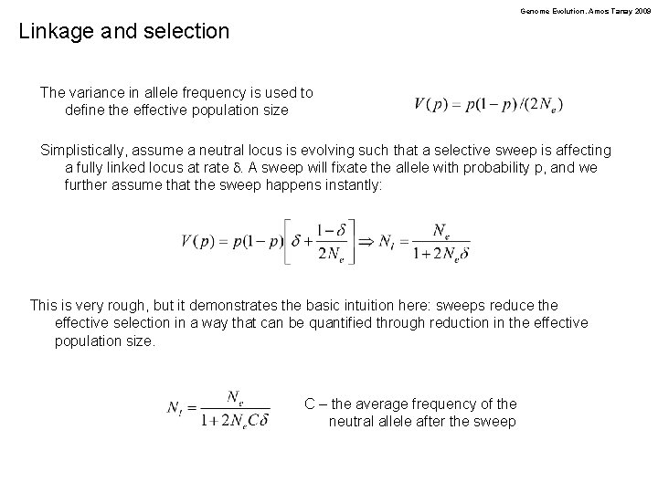
Genome Evolution. Amos Tanay 2009 Linkage and selection The variance in allele frequency is used to define the effective population size Simplistically, assume a neutral locus is evolving such that a selective sweep is affecting a fully linked locus at rate d. A sweep will fixate the allele with probability p, and we further assume that the sweep happens instantly: This is very rough, but it demonstrates the basic intuition here: sweeps reduce the effective selection in a way that can be quantified through reduction in the effective population size. C – the average frequency of the neutral allele after the sweep

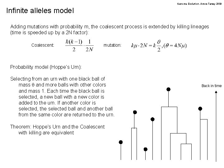
Genome Evolution. Amos Tanay 2009 Infinite alleles model Adding mutations with probability m, the coalescent process is extended by killing lineages (time is speeded up by a 2 N factor): Coalescent: mutation: Probability model (Hoppe’s Urn): Selecting from an urn with one black ball of mass q and more balls with other colors and mass 1. Each time the black ball is selected, a new ball with a new color is added to the urn. If another color is selected, the selected ball and another ball from the same color are returned to the urn. Theorem: Hoppe’s Urn and the Coalescent with killing are equivalent Back in time

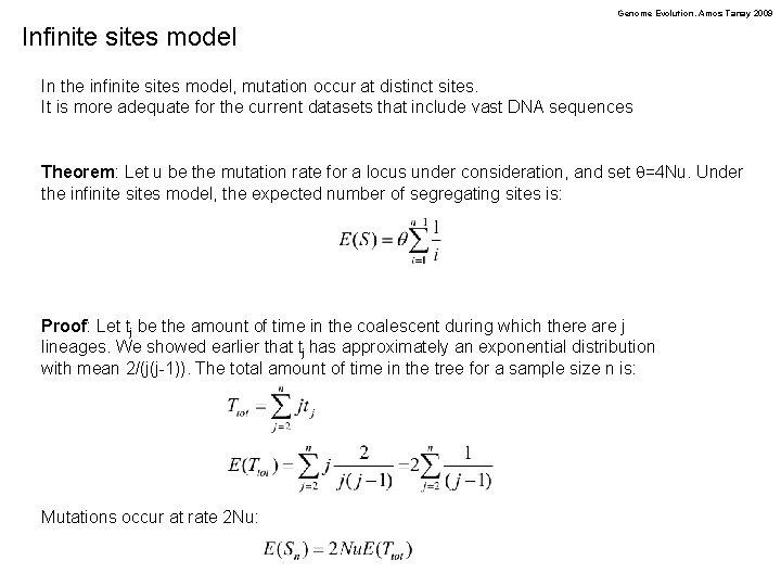
Genome Evolution. Amos Tanay 2009 Infinite sites model In the infinite sites model, mutation occur at distinct sites. It is more adequate for the current datasets that include vast DNA sequences Theorem: Let u be the mutation rate for a locus under consideration, and set q=4 Nu. Under the infinite sites model, the expected number of segregating sites is: Proof: Let tj be the amount of time in the coalescent during which there are j lineages. We showed earlier that tj has approximately an exponential distribution with mean 2/(j(j-1)). The total amount of time in the tree for a sample size n is: Mutations occur at rate 2 Nu:

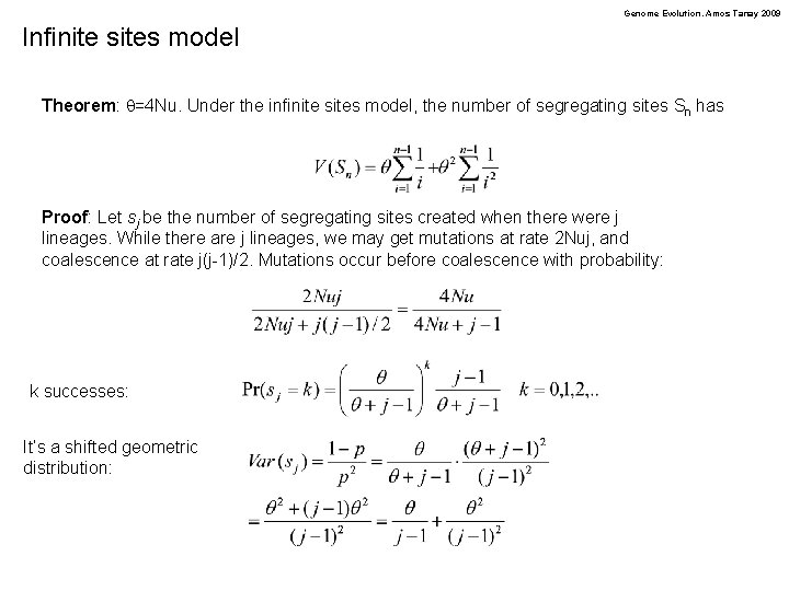
Genome Evolution. Amos Tanay 2009 Infinite sites model Theorem: q=4 Nu. Under the infinite sites model, the number of segregating sites Sn has Proof: Let sj be the number of segregating sites created when there were j lineages. While there are j lineages, we may get mutations at rate 2 Nuj, and coalescence at rate j(j-1)/2. Mutations occur before coalescence with probability: k successes: It’s a shifted geometric distribution:

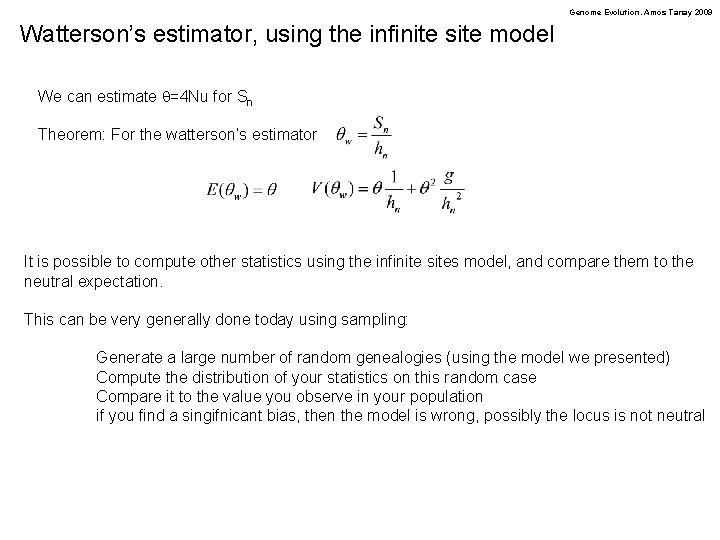
Genome Evolution. Amos Tanay 2009 Watterson’s estimator, using the infinite site model We can estimate q=4 Nu for Sn Theorem: For the watterson’s estimator It is possible to compute other statistics using the infinite sites model, and compare them to the neutral expectation. This can be very generally done today using sampling: Generate a large number of random genealogies (using the model we presented) Compute the distribution of your statistics on this random case Compare it to the value you observe in your population if you find a singifnicant bias, then the model is wrong, possibly the locus is not neutral