Genome Evolution Amos Tanay 2010 Genome evolution Lecture

Genome Evolution. Amos Tanay 2010 Genome evolution Lecture 5: Species, Genomes and Trees

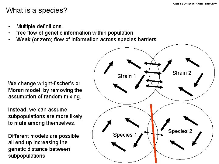
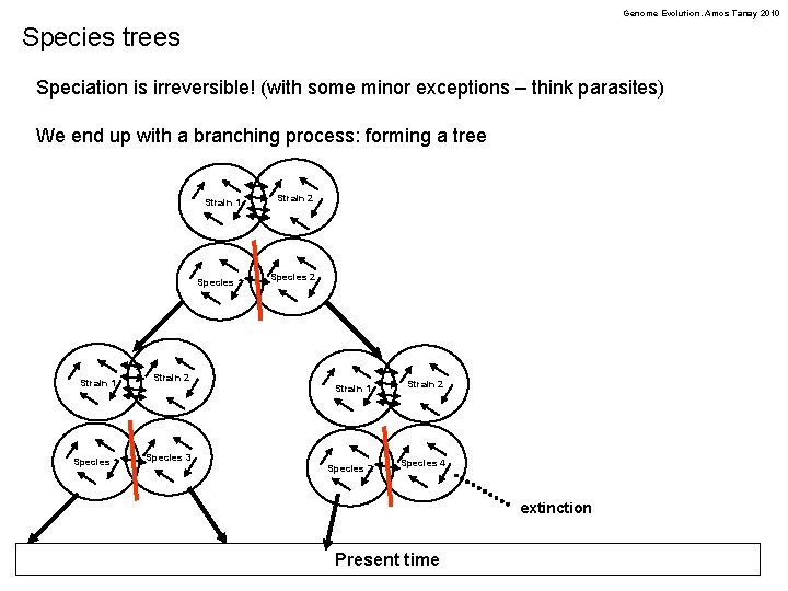
Genome Evolution. Amos Tanay 2010 What is a species? • • • Multiple definitions. . free flow of genetic information within population Weak (or zero) flow of information across species barriers Strain 1 Strain 2 We change wright-fischer’s or Moran model, by removing the assumption of random mixing. Instead, we can assume subpopulations are more likely to mate among themselves. Different models are possible, all end up increasing the genetic distance between subpopulations Species 1 Species 2

Genome Evolution. Amos Tanay 2010 Speciation The Phenomenon of new species emergence is called speciation It is well accepted that speciation is driven by the formation of reproductive barriers Allopatric speciation – occurs through geographical separation Parapatric speciation – occurs without geographical separation but with weak flow of genetic information Sympatric speciation – occurs while information is flowing Barriers can genetic, physical, and behavioral

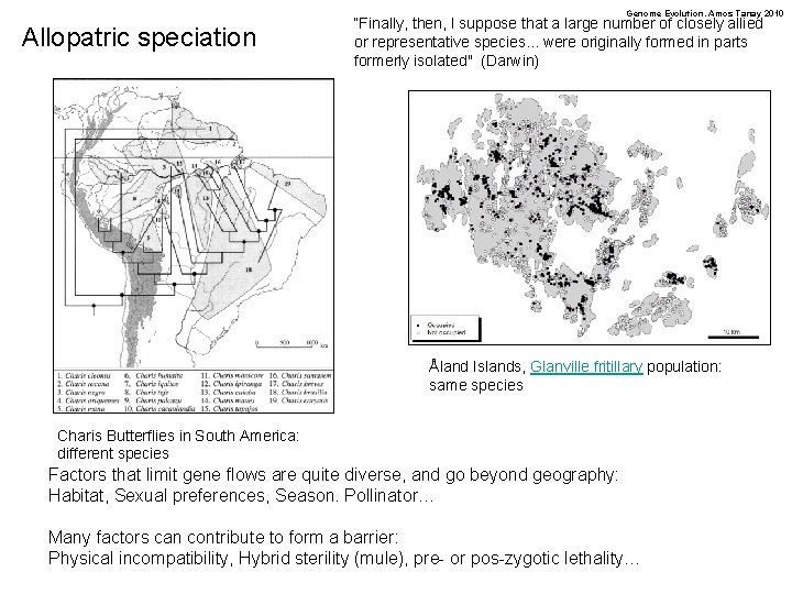
Genome Evolution. Amos Tanay 2010 Allopatric speciation “Finally, then, I suppose that a large number of closely allied or representative species. . . were originally formed in parts formerly isolated" (Darwin) Åland Islands, Glanville fritillary population: same species Charis Butterflies in South America: different species Factors that limit gene flows are quite diverse, and go beyond geography: Habitat, Sexual preferences, Season. Pollinator… Many factors can contribute to form a barrier: Physical incompatibility, Hybrid sterility (mule), pre- or pos-zygotic lethality…

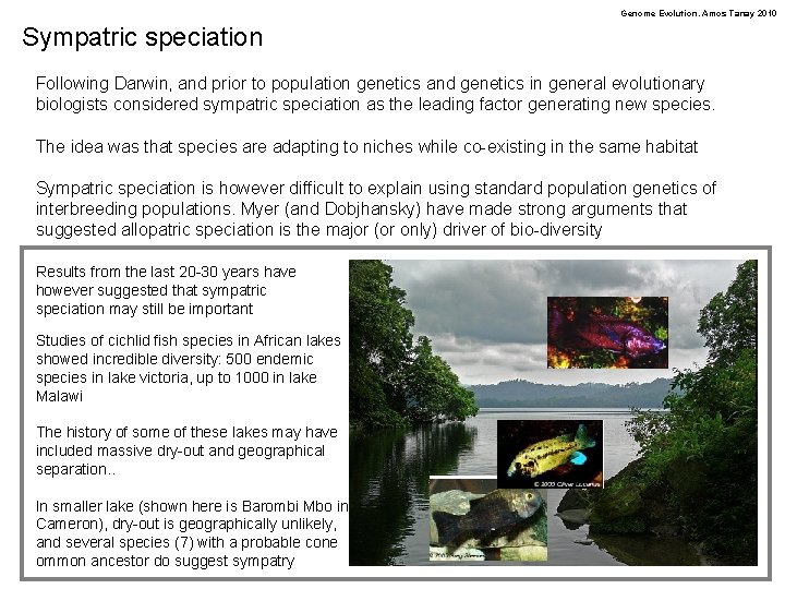
Genome Evolution. Amos Tanay 2010 Sympatric speciation Following Darwin, and prior to population genetics and genetics in general evolutionary biologists considered sympatric speciation as the leading factor generating new species. The idea was that species are adapting to niches while co-existing in the same habitat Sympatric speciation is however difficult to explain using standard population genetics of interbreeding populations. Myer (and Dobjhansky) have made strong arguments that suggested allopatric speciation is the major (or only) driver of bio-diversity Results from the last 20 -30 years have however suggested that sympatric speciation may still be important Studies of cichlid fish species in African lakes showed incredible diversity: 500 endemic species in lake victoria, up to 1000 in lake Malawi The history of some of these lakes may have included massive dry-out and geographical separation. . In smaller lake (shown here is Barombi Mbo in Cameron), dry-out is geographically unlikely, and several species (7) with a probable cone ommon ancestor do suggest sympatry

Genome Evolution. Amos Tanay 2010 Species trees Speciation is irreversible! (with some minor exceptions – think parasites) We end up with a branching process: forming a tree Strain 1 Strain 2 Species 1 Species 3 Strain 1 Strain 2 Species 1 Species 2 Strain 1 Strain 2 Species 4 extinction Present time

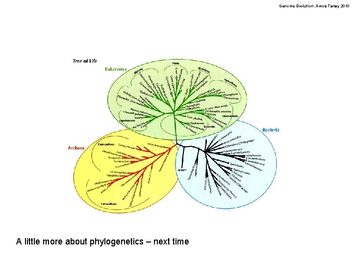
Genome Evolution. Amos Tanay 2010 A little more about phylogenetics – next time

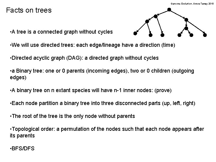
Genome Evolution. Amos Tanay 2010 Facts on trees • A tree is a connected graph without cycles • We will use directed trees: each edge/lineage have a direction (time) • Directed acyclic graph (DAG): a directed graph without cycles • a Binary tree: one or 0 parents (incoming edges), two or 0 children (outgoing edges) • A binary tree on n extant species will have n-1 inner nodes: (prove) • Each node partition a binary tree into three disconnected parts (up, left, right) • The root of the tree is the only node without parents • Topological order: a permutation of the nodes such that each node appears after its parents • BFS/DFS

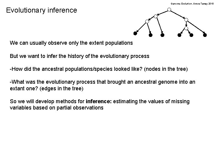
Genome Evolution. Amos Tanay 2010 Evolutionary inference We can usually observe only the extent populations But we want to infer the history of the evolutionary process -How did the ancestral populations/species looked like? (nodes in the tree) -What was the evolutionary process that brought an ancestral genome into an extant one? (edges in the tree) So we will develop methods for inference: estimating the values of missing variables based on partial observations

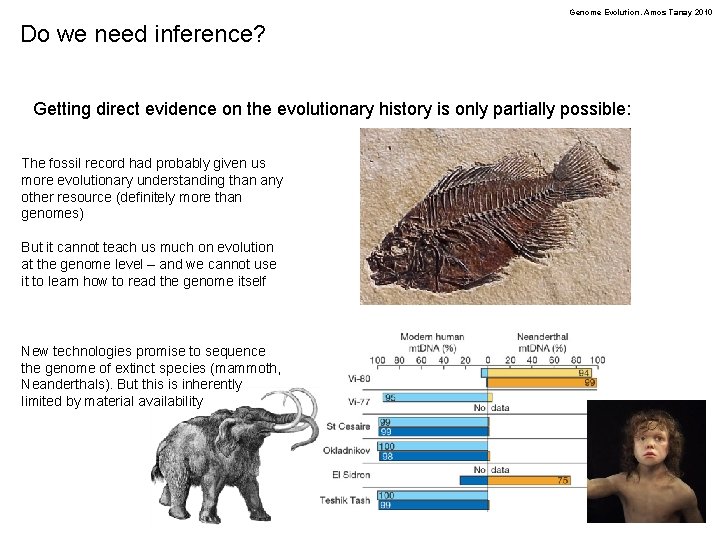
Genome Evolution. Amos Tanay 2010 Do we need inference? Getting direct evidence on the evolutionary history is only partially possible: The fossil record had probably given us more evolutionary understanding than any other resource (definitely more than genomes) But it cannot teach us much on evolution at the genome level – and we cannot use it to learn how to read the genome itself New technologies promise to sequence the genome of extinct species (mammoth, Neanderthals). But this is inherently limited by material availability

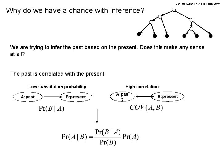
Genome Evolution. Amos Tanay 2010 Why do we have a chance with inference? We are trying to infer the past based on the present. Does this make any sense at all? The past is correlated with the present Low substitution probability A: past B: present High correlation A: pas t B: present

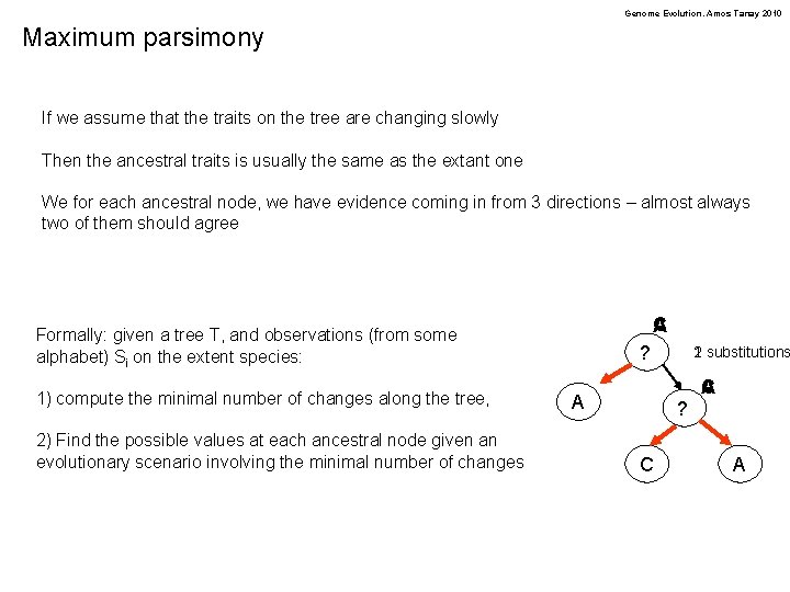
Genome Evolution. Amos Tanay 2010 Maximum parsimony If we assume that the traits on the tree are changing slowly Then the ancestral traits is usually the same as the extant one We for each ancestral node, we have evidence coming in from 3 directions – almost always two of them should agree C A Formally: given a tree T, and observations (from some alphabet) Si on the extent species: 1) compute the minimal number of changes along the tree, 2) Find the possible values at each ancestral node given an evolutionary scenario involving the minimal number of changes ? A 2 substitutions 1 ? C C A A

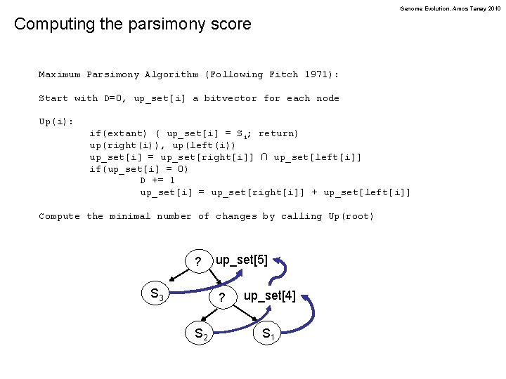
Genome Evolution. Amos Tanay 2010 Computing the parsimony score Maximum Parsimony Algorithm (Following Fitch 1971): Start with D=0, up_set[i] a bitvector for each node Up(i): if(extant) { up_set[i] = Si; return} up(right(i)), up(left(i)) up_set[i] = up_set[right[i]] ∩ up_set[left[i]] if(up_set[i] = 0) D += 1 up_set[i] = up_set[right[i]] + up_set[left[i]] Compute the minimal number of changes by calling Up(root) ? S 3 up_set[5] ? S 2 up_set[4] S 1

Genome Evolution. Amos Tanay 2010 Parsimony “inference” ? up_set[3] S 3 down_set[5] ? S 2 down_set[4] S 1 Set[i] = up_set[i] ∩ down_set[i] Algorithm (Following Fitch 1971): Up(i): if(extant) { up_set[i] = Si; return} up(right(i)), up(left(i)) up_set[i] = up_set[right[i]] ∩ up_set[left[i]] if(up_set[i] = 0) D += 1 up_set[i] = up_set[right[i]] + up_set[left[i]] Down(i): down_set[i] = up_set[sib[i]] ∩ down_set[par(i)] if(down_set[i] = 0) { down_set[i] = up_set[sib[i]] + down_set[par(i)] } down(left(i)), down(right(i)) Algorithm: D=0 up(root); down_set[root] = 0; down(right(root)); down(left(root));

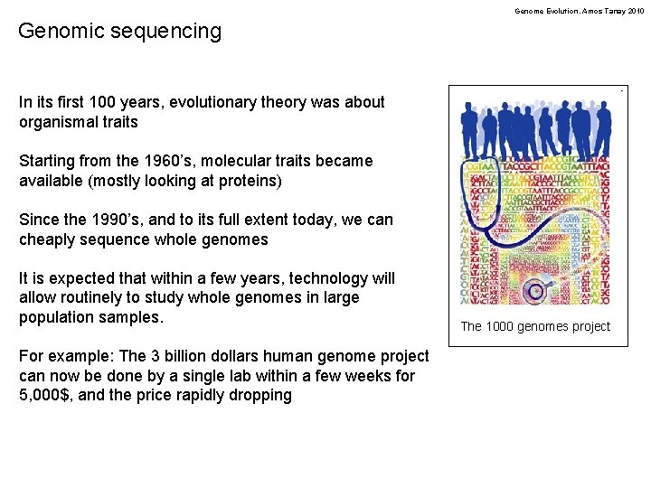
Genome Evolution. Amos Tanay 2010 Genomic sequencing In its first 100 years, evolutionary theory was about organismal traits Starting from the 1960’s, molecular traits became available (mostly looking at proteins) Since the 1990’s, and to its full extent today, we can cheaply sequence whole genomes It is expected that within a few years, technology will allow routinely to study whole genomes in large population samples. For example: The 3 billion dollars human genome project can now be done by a single lab within a few weeks for 5, 000$, and the price rapidly dropping The 1000 genomes project

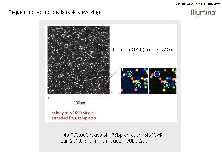
Genome Evolution. Amos Tanay 2010 Sequencing technology is rapidly evolving: Illumina GAII (here at WIS) ~40, 000 reads of ~36 bp on each, 5 k-10 k$ Jan 2010: 300 million reads, 150 bpx 2…

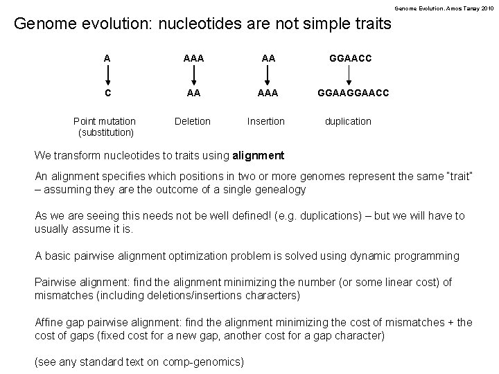
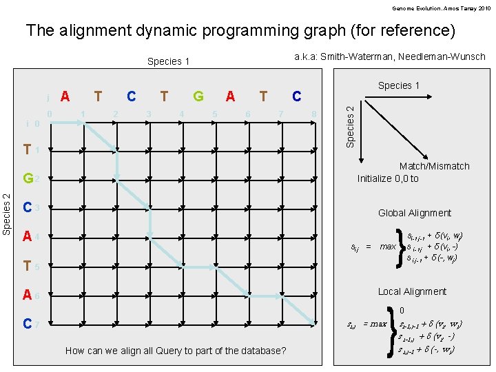
Genome Evolution. Amos Tanay 2010 Genome evolution: nucleotides are not simple traits A AA C AA AAA Deletion Insertion Point mutation (substitution) GGAACC duplication We transform nucleotides to traits using alignment An alignment specifies which positions in two or more genomes represent the same “trait” – assuming they are the outcome of a single genealogy As we are seeing this needs not be well defined! (e. g. duplications) – but we will have to usually assume it is. A basic pairwise alignment optimization problem is solved using dynamic programming Pairwise alignment: find the alignment minimizing the number (or some linear cost) of mismatches (including deletions/insertions characters) Affine gap pairwise alignment: find the alignment minimizing the cost of mismatches + the cost of gaps (fixed cost for a new gap, another cost for a gap character) (see any standard text on comp-genomics)

Genome Evolution. Amos Tanay 2010 The alignment dynamic programming graph (for reference) a. k. a: Smith-Waterman, Needleman-Wunsch Species 1 0 A T 1 C 2 T 3 G 4 A 5 T 6 C 7 i 0 Species 2 T 1 8 Species 2 j Species 1 G 2 Match/Mismatch Initialize 0, 0 to C 3 Global Alignment A 4 si, j = si-1, j-1 + δ (vi, wj) s i-1, j + δ (vi, -) s i, j-1 + δ (-, wj) max T 5 Local Alignment A 6 si, j = max C 7 How can we align all Query to part of the database? 0 si-1, j-1 + δ (vi, wj) s i-1, j + δ (vi, -) s i, j-1 + δ (-, wj)

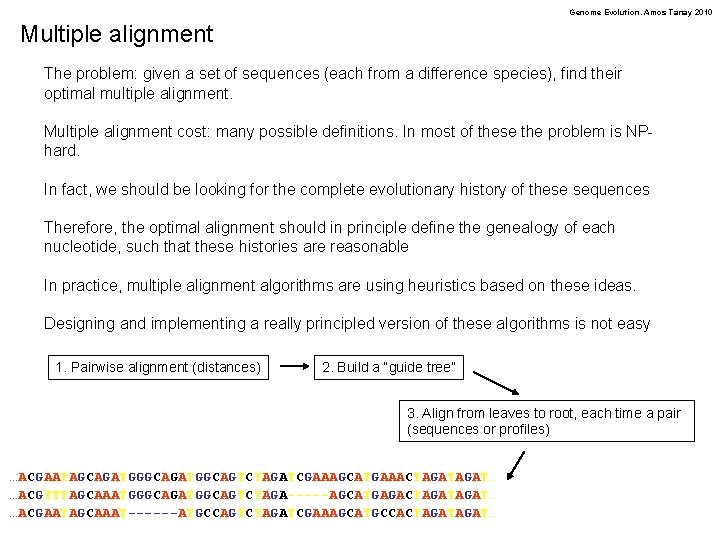
Genome Evolution. Amos Tanay 2010 Multiple alignment The problem: given a set of sequences (each from a difference species), find their optimal multiple alignment. Multiple alignment cost: many possible definitions. In most of these the problem is NPhard. In fact, we should be looking for the complete evolutionary history of these sequences Therefore, the optimal alignment should in principle define the genealogy of each nucleotide, such that these histories are reasonable In practice, multiple alignment algorithms are using heuristics based on these ideas. Designing and implementing a really principled version of these algorithms is not easy 1. Pairwise alignment (distances) 2. Build a “guide tree” 3. Align from leaves to root, each time a pair (sequences or profiles) …ACGAATAGCAGATGGCAGTCTAGATCGAAAGCATGAAACTAGAT… …ACGTTTAGCAAATGGGCAGATGGCAGTCTAGA-----AGCATGAGACTAGAT… …ACGAATAGCAAAT------ATGCCAGTCTAGATCGAAAGCATGCCACTAGAT…

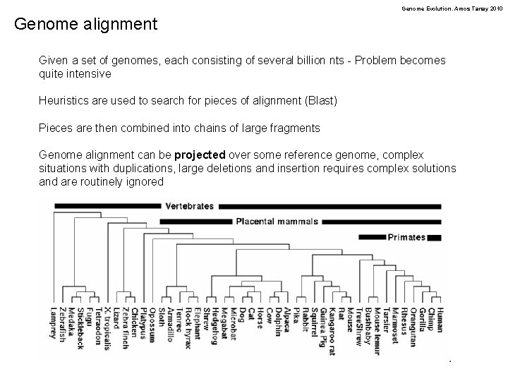
Genome Evolution. Amos Tanay 2010 Genome alignment Given a set of genomes, each consisting of several billion nts - Problem becomes quite intensive Heuristics are used to search for pieces of alignment (Blast) Pieces are then combined into chains of large fragments Genome alignment can be projected over some reference genome, complex situations with duplications, large deletions and insertion requires complex solutions and are routinely ignored