L 1 Trigger Rate Study Nathaniel Amos 1

L 1 Trigger Rate Study Nathaniel Amos 1

Part 1 • GMT Eta Distributions 2

GMT Eta Distribution • Studied Eta distribution of GMT output • Can be used to estimate GMT Rate in Eta • Data sample taken from: – Runs: 190389 -194115 – HLT_L 1 Single. Mu. Open and json_DSConly. txt • GMT Qualities selected: – Quality 5: RPC Only – Quality 6: DT or CSC, No RPC – Quality 7: DT/RPC or CSC/RPC 3

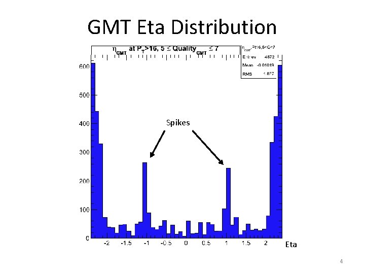
GMT Eta Distribution Spikes Eta 4

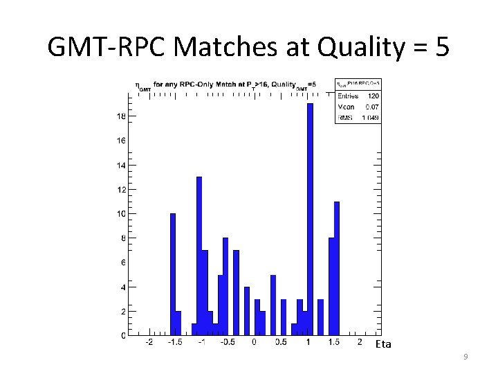
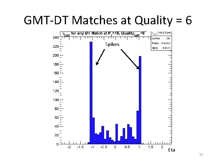
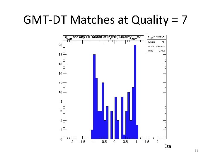
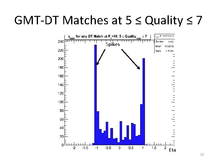
What causes the spikes? • Observe each subsystem independently – Observe GMT-DT matches at GMT Quality 6, 7 – Observe GMT-CSC matches at GMT Quality 6, 7 • If GMT Eta > 2. 1, require CSCTF Mode 5 – Observe RPC-GMT matches at GMT Quality 5 and GMT BX = 0 • Plot each Eta distribution 5

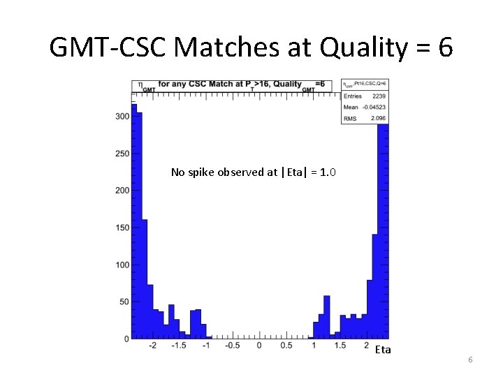
GMT-CSC Matches at Quality = 6 No spike observed at |Eta| = 1. 0 Eta 6

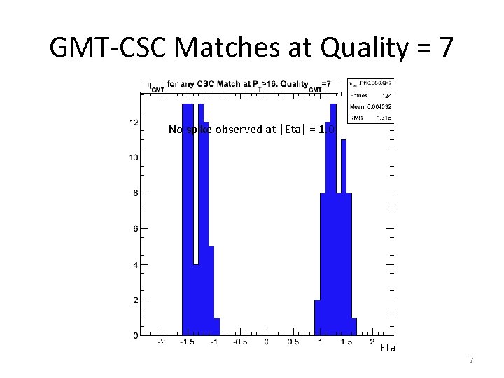
GMT-CSC Matches at Quality = 7 No spike observed at |Eta| = 1. 0 Eta 7

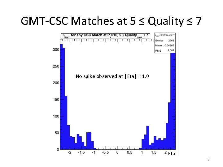
GMT-CSC Matches at 5 ≤ Quality ≤ 7 No spike observed at |Eta| = 1. 0 Eta 8

GMT-RPC Matches at Quality = 5 Eta 9

GMT-DT Matches at Quality = 6 Spikes Eta 10

GMT-DT Matches at Quality = 7 Eta 11

GMT-DT Matches at 5 ≤ Quality ≤ 7 Spikes Eta 12

Part 2 • GMT Relative Rates 13

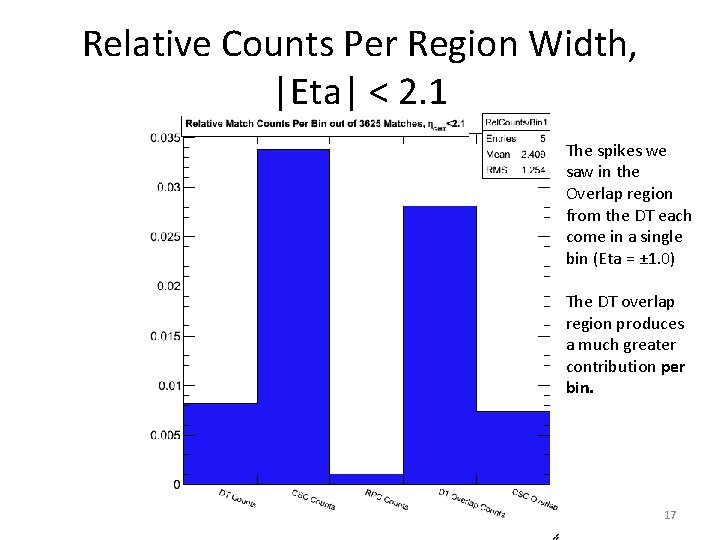
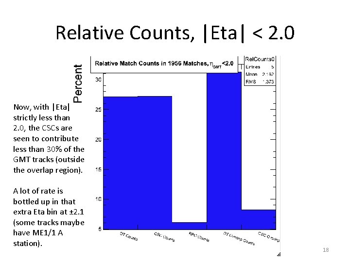
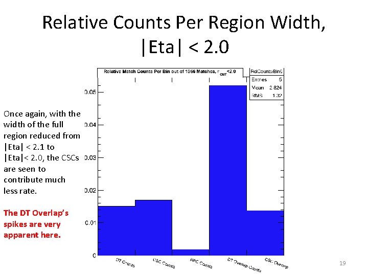
Relative GMT Matches • Plot number of GMT-subsystem matches relative to total number of GMT matches – Plotted for each category (below) • Define several categories for matches: – DT, |Eta| < 0. 9 – CSC, 1. 2 < |Eta| < 2. 1 • or 1. 2 < |Eta| < 2. 0 (See next slides) – RPC, |Eta| < 1. 6 – DT Overlap, 0. 9 < |Eta| < 1. 2 – CSC Overlap, 0. 9 < |Eta| < 1. 2 14

Two Methods of Plotting • Plot GMT-subsystem matches divided by total number of GMT matches (referred to as “relative counts”) • Plot GMT-subsystem matches divided by total number of GMT matches per subsystem region width (a type of rate density) – Example: • CSC (1. 2 < |Eta| < 2. 1): each Eta bin has width of Eta = 0. 1 • Therefore CSC relative counts divided by 18 bins 15

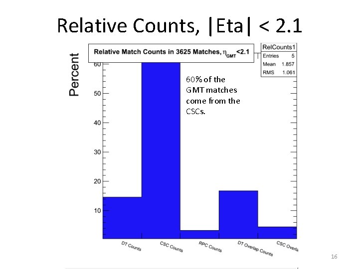
Relative Counts, |Eta| < 2. 1 60% of the GMT matches come from the CSCs. 16

Relative Counts Per Region Width, |Eta| < 2. 1 The spikes we saw in the Overlap region from the DT each come in a single bin (Eta = ± 1. 0) The DT overlap region produces a much greater contribution per bin. 17

Relative Counts, |Eta| < 2. 0 Now, with |Eta| strictly less than 2. 0, the CSCs are seen to contribute less than 30% of the GMT tracks (outside the overlap region). A lot of rate is bottled up in that extra Eta bin at ± 2. 1 (some tracks maybe have ME 1/1 A station). 18

Relative Counts Per Region Width, |Eta| < 2. 0 Once again, with the width of the full region reduced from |Eta| < 2. 1 to |Eta|< 2. 0, the CSCs are seen to contribute much less rate. The DT Overlap’s spikes are very apparent here. 19

Conclusions • Spikes do not appear to come from CSC – But there is a lot of rate at 2. 0 <|Eta| < 2. 1 • Some tracks may come from ME 1/1 A • DT in overlap region shows spikes – Appears to be Eta = ± 1. 0 • Plan to repeat study – Use HLT_L 1 Single. Mu 10 • More statistics – JSON_Muon. Phys. txt • Exclude possible problems in muon system 20