Gaussian Mixture Models And their training with the

Gaussian Mixture Models And their training with the EM algorithm

Introduction We saw how to fit Gaussian curves on data samples But the Gaussian curve as a model is not really a flexible The distribution of real data rarely have a Gaussian shape So the „model error” will be large Today we introduce a new model called the Gaussian Mixture Model It has a much more flexible shape than a simple Gaussian But, unfortunately, it will be much more difficult to train We will use the Maximum likelihood target function, as before But, instead of a closed form solution, we will introduce an iterative algorithm to optimize its parameters. This will be the EM algorithm We will again train the model of the different classes separately So we will talk about how to fit the model on the samples of one class, and drop the condition ci from the notation but don’t forget that the process should be repeated for all classes

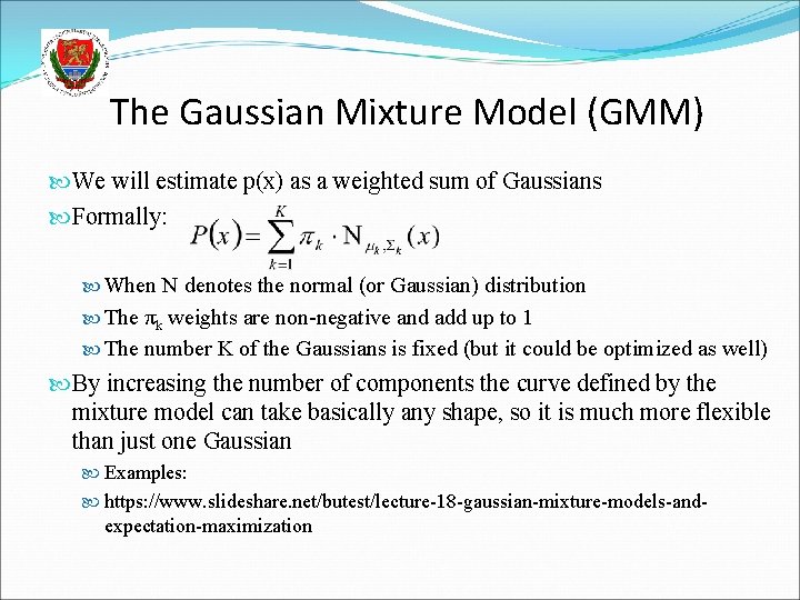
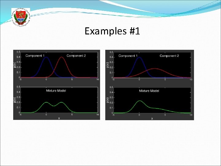
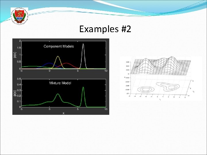
The Gaussian Mixture Model (GMM) We will estimate p(x) as a weighted sum of Gaussians Formally: When N denotes the normal (or Gaussian) distribution The πk weights are non-negative and add up to 1 The number K of the Gaussians is fixed (but it could be optimized as well) By increasing the number of components the curve defined by the mixture model can take basically any shape, so it is much more flexible than just one Gaussian Examples: https: //www. slideshare. net/butest/lecture-18 -gaussian-mixture-models-and- expectation-maximization

Examples #1

Examples #2

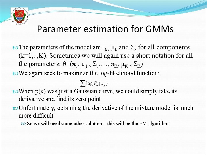
Parameter estimation for GMMs The parameters of the model are πk , μk and Σk for all components (k=1, . . , K). Sometimes we will again use a short notation for all the parameters: θ=(π1, μ 1 , 1, …, πK, μK , K) We again seek to maximize the log-likelihood function: When p(x) was just a Gaussian curve, we could simply take its derivative and find its zero point Unfortunately, obtaining the derivative of the mixture model is much more difficult So we will need some other solution – this will be the EM algorithm

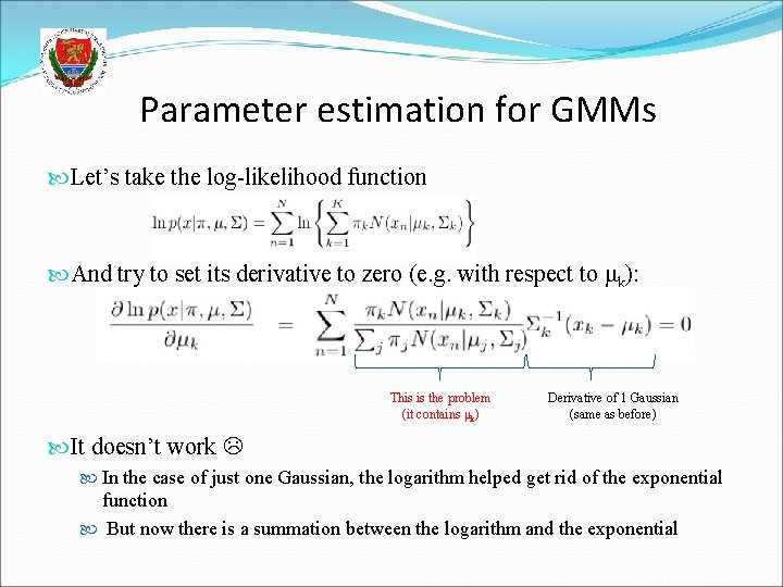
Parameter estimation for GMMs Let’s take the log-likelihood function And try to set its derivative to zero (e. g. with respect to μk): This is the problem (it contains μk) Derivative of 1 Gaussian (same as before) It doesn’t work In the case of just one Gaussian, the logarithm helped get rid of the exponential function But now there is a summation between the logarithm and the exponential

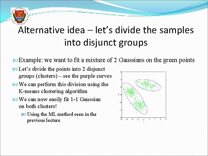
Alternative idea – let’s divide the samples into disjunct groups Example: we want to fit a mixture of 2 Gaussians on the green points Let’s divide the points into 2 disjunct groups (clusters) – see the purple curves We can perform this division using the K-means clustering algorithm We can now easily fit 1 -1 Gaussian on both clusters! Using the ML method seen in the previous lecture

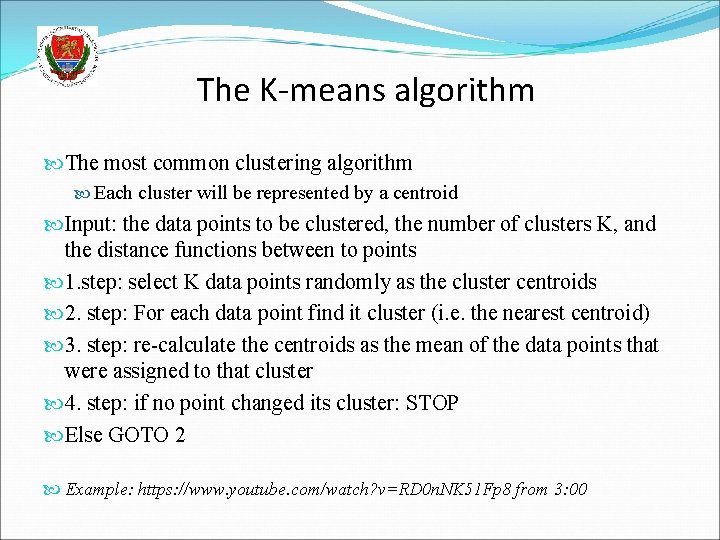
The K-means algorithm The most common clustering algorithm Each cluster will be represented by a centroid Input: the data points to be clustered, the number of clusters K, and the distance functions between to points 1. step: select K data points randomly as the cluster centroids 2. step: For each data point find it cluster (i. e. the nearest centroid) 3. step: re-calculate the centroids as the mean of the data points that were assigned to that cluster 4. step: if no point changed its cluster: STOP Else GOTO 2 Example: https: //www. youtube. com/watch? v=RD 0 n. NK 51 Fp 8 from 3: 00

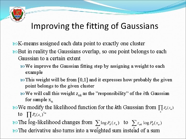
Improving the fitting of Gaussians K-means assigned each data point to exactly one cluster But in reality the Gaussians overlap, so one point belongs to each Gaussian to a certain extent We improve the Gaussian fitting step by assigning a weight to each example This weight will be from [0, 1] and it expresses how probably the given point belongs to the given cluster We will call this weight znk as the ”responsibility” of the kth Gaussian for sample xn We modify the likelihood function for the kth Gaussian from to The log-likelihood changes from to The derivative also turns into a weighted sum instead of a sum

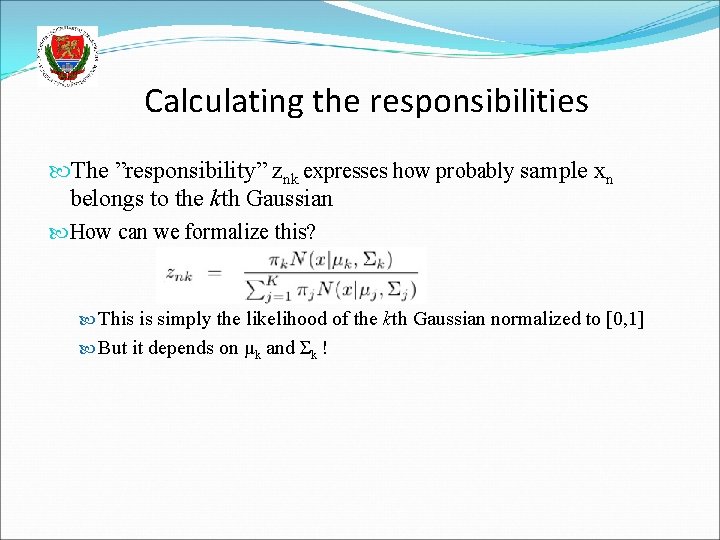
Calculating the responsibilities The ”responsibility” znk expresses how probably sample xn belongs to the kth Gaussian How can we formalize this? This is simply the likelihood of the kth Gaussian normalized to [0, 1] But it depends on μk and Σk !

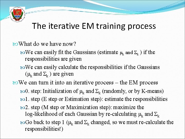
The iterative EM training process What do we have now? We can easily fit the Gaussians (estimate μk and Σk ) if the responsibilities are given We can easily calculate the responsibilities if the Gaussians (μk and Σk ) are given We can turn it into an iterative process – the EM process 0. step: Initialization of μk and Σk (randomly, or by K-means) 1. step (E step or Estimation step): estimate the responsibilities 2. step (M step or Maximization step): maximize the log-likelihood of each Gaussian by re-calculating μk and Σk Go back to step 1 (μk and Σk changed, so we must re-calculate the responsibilities!)

Alternative explanation Remember that we tried to take the derivative of the loglikelihood of the mixture model, but we got stuck: This was the problem (it contains μk) Notice that the problematic part is equivalent with what we called the “responsibility”! Let’s cheat, and act as if it was a constant, independent of μk! Then we can easily calculate the derivative and obtain a new estimate for μk (and the same will be true for Σk) But what we obtained won’t be optimal, as we cheated So we re-calculate the responsibilites and repeat the whole process again (and again)

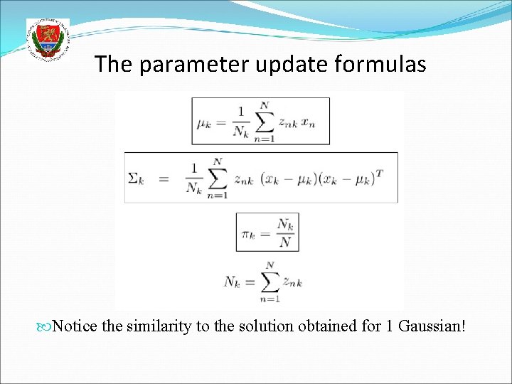
The parameter update formulas Notice the similarity to the solution obtained for 1 Gaussian!

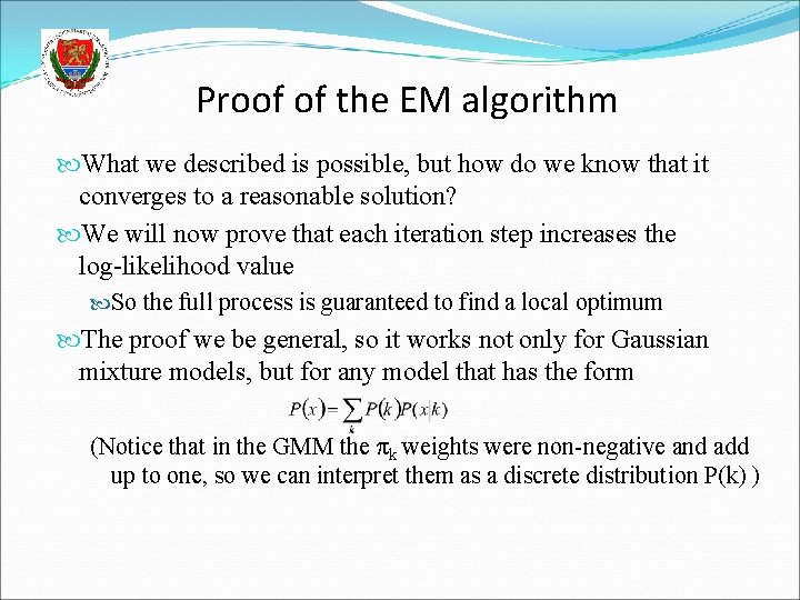
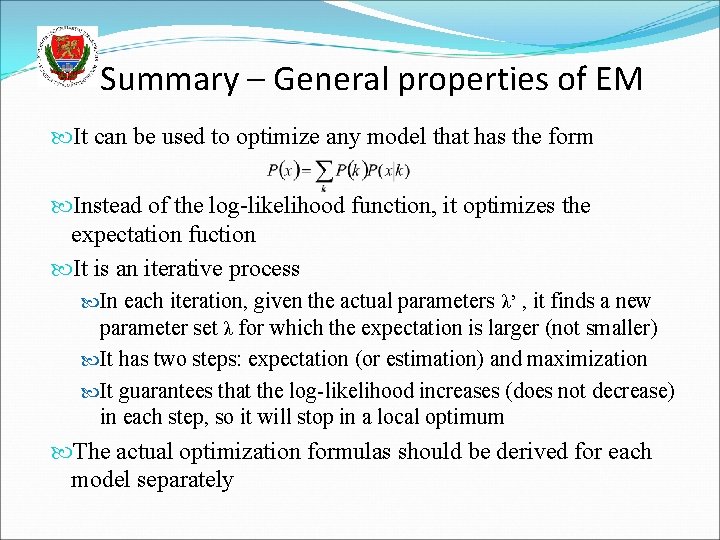
Proof of the EM algorithm What we described is possible, but how do we know that it converges to a reasonable solution? We will now prove that each iteration step increases the log-likelihood value So the full process is guaranteed to find a local optimum The proof we be general, so it works not only for Gaussian mixture models, but for any model that has the form (Notice that in the GMM the πk weights were non-negative and add up to one, so we can interpret them as a discrete distribution P(k) )

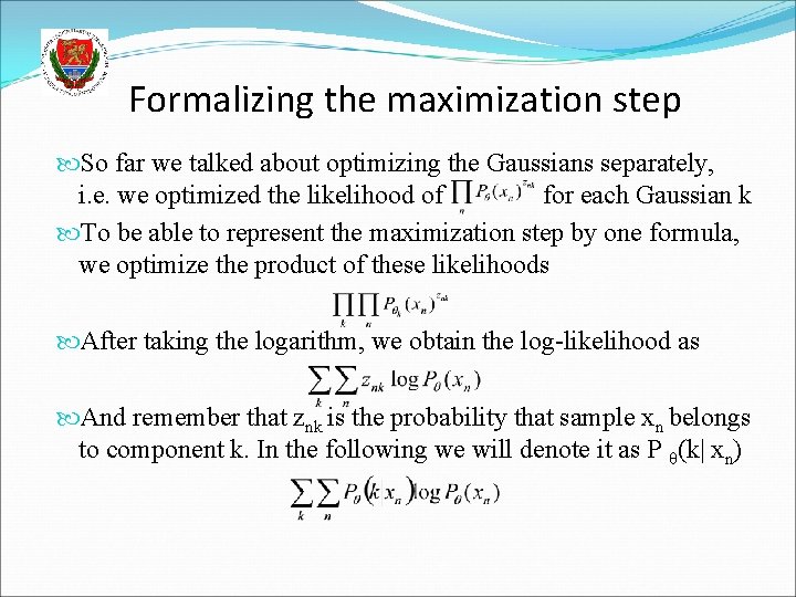
Formalizing the maximization step So far we talked about optimizing the Gaussians separately, i. e. we optimized the likelihood of for each Gaussian k To be able to represent the maximization step by one formula, we optimize the product of these likelihoods After taking the logarithm, we obtain the log-likelihood as And remember that znk is the probability that sample xn belongs to component k. In the following we will denote it as P θ(k| xn)

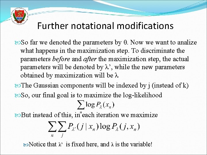
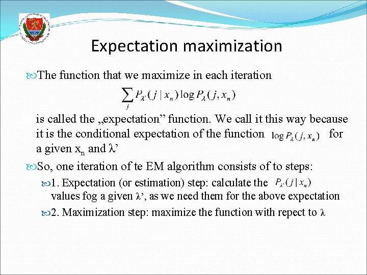
Further notational modifications So far we denoted the parameters by θ. Now we want to analize what happens in the maximization step. To discriminate the parameters before and after the maximization step, the actual parameters will be denoted by λ’, while the new parameters obtained by maximization will be λ The Gaussian components will be indexed by j (instead of k) So, our final goal is to maximize the log-likelihood But instead of this, in each iteration we maximize Notice that λ’ is fixed here, and λ is the variable!

Expectation maximization The function that we maximize in each iteration is called the „expectation” function. We call it this way because it is the conditional expectation of the function for a given xn and λ’ So, one iteration of te EM algorithm consists of to steps: 1. Expectation (or estimation) step: calculate the values fog a given λ’, as we need them for the above expectation 2. Maximization step: maximize the function with repect to λ

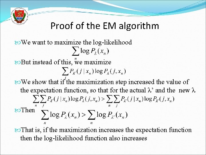
Proof of the EM algorithm We want to maximize the log-likelihood But instead of this, we maximize We show that if the maximization step increased the value of the expectation function, so that for the actual λ’ and the new λ Then That is, if the maximization increases the expectation function the log-likelihood function also increases

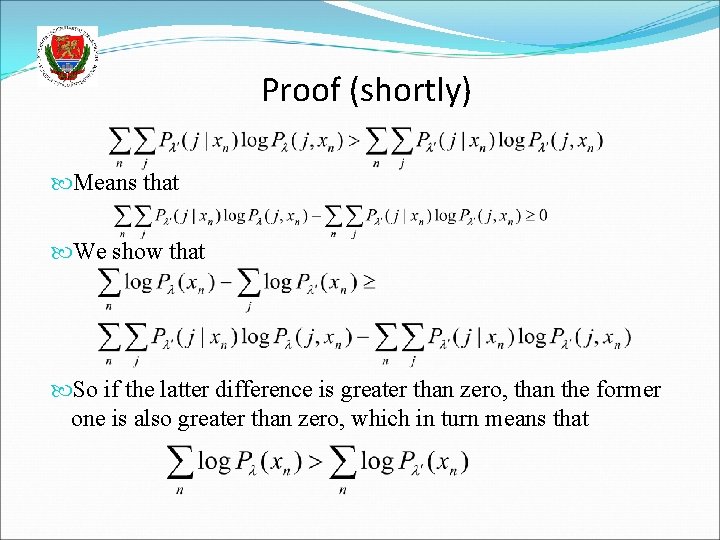
Proof (shortly) Means that We show that So if the latter difference is greater than zero, than the former one is also greater than zero, which in turn means that

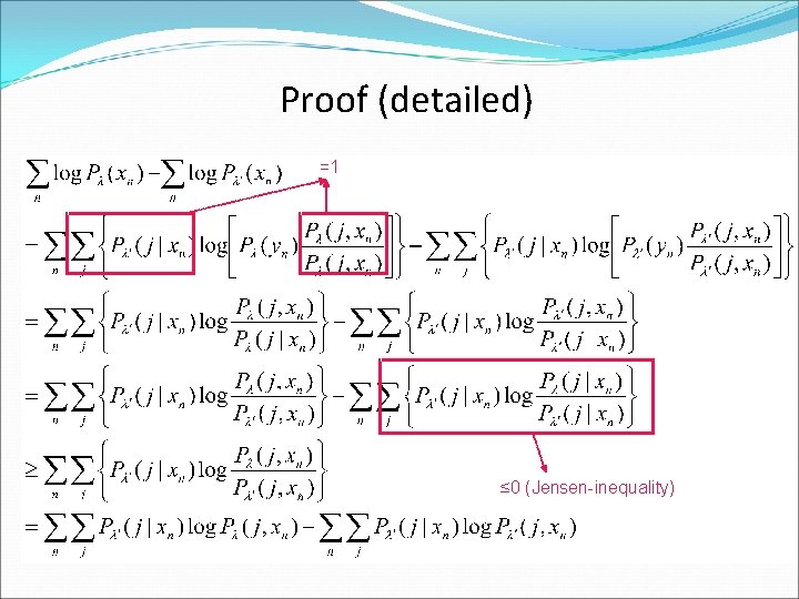
Proof (detailed) =1 ≤ 0 (Jensen-inequality)

The Jensen inequality In general, for any p(x) and q(x) distributions: Specifically, in this case:

Summary – General properties of EM It can be used to optimize any model that has the form Instead of the log-likelihood function, it optimizes the expectation fuction It is an iterative process In each iteration, given the actual parameters λ’ , it finds a new parameter set λ for which the expectation is larger (not smaller) It has two steps: expectation (or estimation) and maximization It guarantees that the log-likelihood increases (does not decrease) in each step, so it will stop in a local optimum The actual optimization formulas should be derived for each model separately

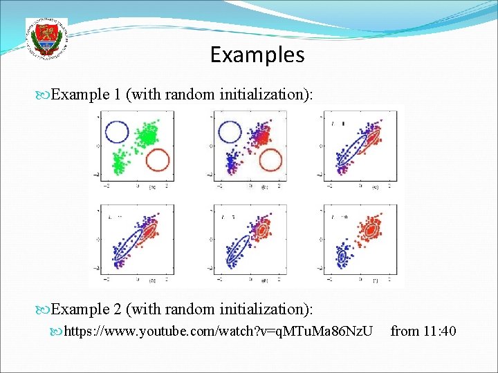
Examples Example 1 (with random initialization): Example 2 (with random initialization): https: //www. youtube. com/watch? v=q. MTu. Ma 86 Nz. U from 11: 40

Some technical remarks The parameters are usually initialized via K-means clustering It may give quite different results depending to the initial choice of the centroids So the clustering process is worth repeating with various initial choice (e. g. random choice) of the centroids Then we start the EM process with the clustering result that gives the largest initial likelihood value Of course, there exist more sophisticated methods to initialize the centroids

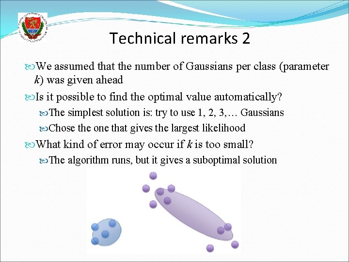
Technical remarks 2 We assumed that the number of Gaussians per class (parameter k) was given ahead Is it possible to find the optimal value automatically? The simplest solution is: try to use 1, 2, 3, … Gaussians Chose the one that gives the largest likelihood What kind of error may occur if k is too small? The algorithm runs, but it gives a suboptimal solution

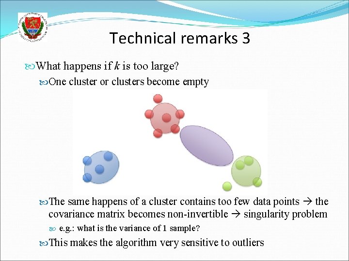
Technical remarks 3 What happens if k is too large? One cluster or clusters become empty The same happens of a cluster contains too few data points the covariance matrix becomes non-invertible singularity problem e. g. : what is the variance of 1 sample? This makes the algorithm very sensitive to outliers

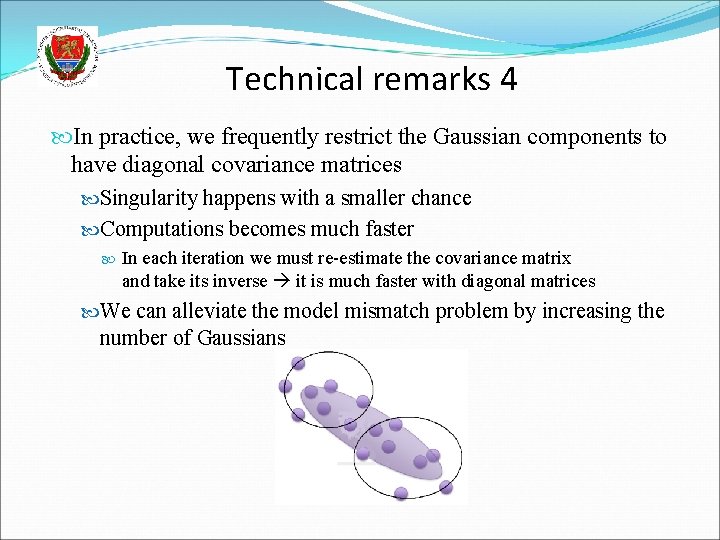
Technical remarks 4 In practice, we frequently restrict the Gaussian components to have diagonal covariance matrices Singularity happens with a smaller chance Computations becomes much faster In each iteration we must re-estimate the covariance matrix and take its inverse it is much faster with diagonal matrices We can alleviate the model mismatch problem by increasing the number of Gaussians