Statistical Characterization Using Automatic Learning Gaussian Mixture Models

Statistical Characterization Using Automatic Learning Gaussian Mixture Models in Diamond M Field, TX David Lubo*, The University of Oklahoma, Simon Bolivar University Vikram Jayaram, The University of Oklahoma Kurt J. Marfurt, The University of Oklahoma

RESEARCH OBJECTIVE Ø In a situation when we have thousands of wells in a resource play, the propose workflow can determine which wells are alike and which are different. We can also deduce if is there a correlation to those that are alike or different to know where we have good EUR.

OUTLINE § Problem Statement: Unsupervised classification using GMM § Gaussian Mixture Models (GMM) § Independent Component Analysis (ICA) § Geological Setting: Diamond M Field § Statistical Characterization using GMM § Study conclusions

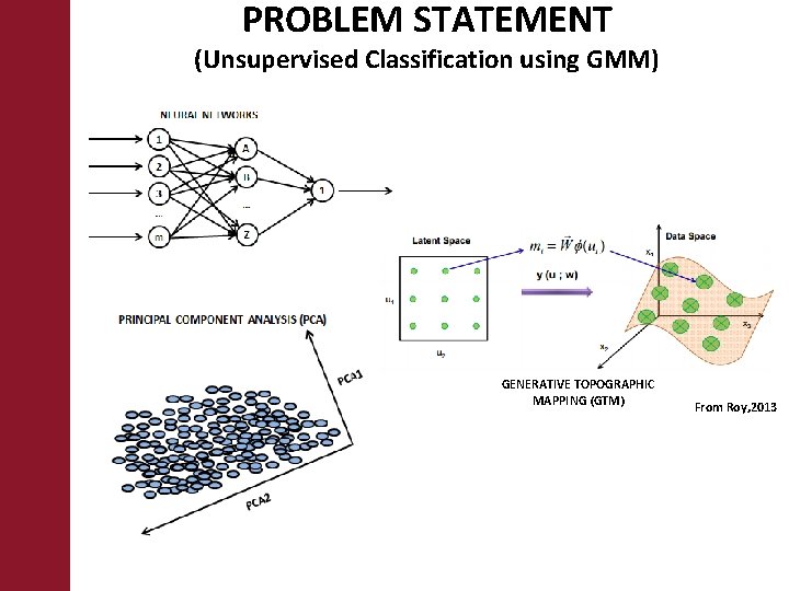
PROBLEM STATEMENT (Unsupervised Classification using GMM) GENERATIVE TOPOGRAPHIC MAPPING (GTM) From Roy, 2013

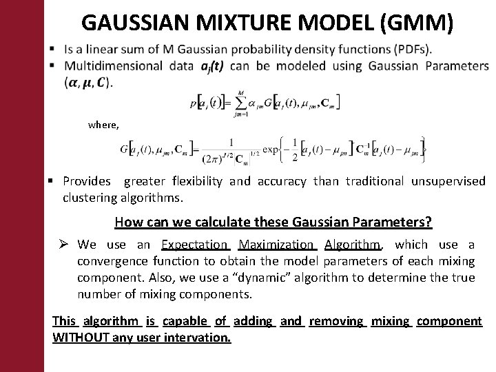
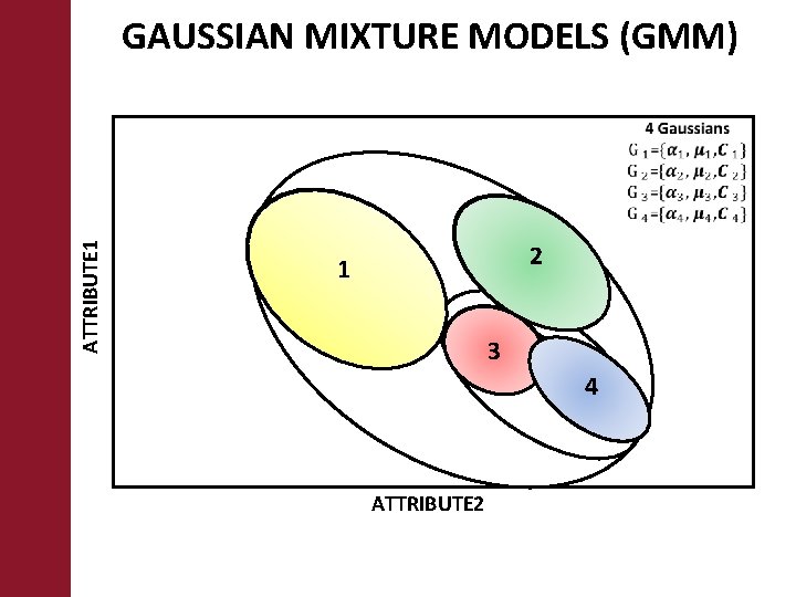
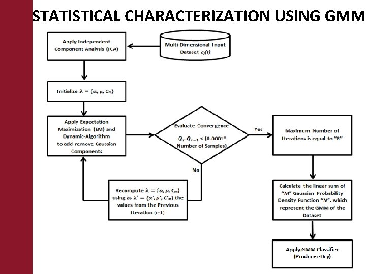
GAUSSIAN MIXTURE MODEL (GMM) where, § Provides greater flexibility and accuracy than traditional unsupervised clustering algorithms. How can we calculate these Gaussian Parameters? Ø We use an Expectation Maximization Algorithm, which use a convergence function to obtain the model parameters of each mixing component. Also, we use a “dynamic” algorithm to determine the true number of mixing components. This algorithm is capable of adding and removing mixing component WITHOUT any user intervation.

ATTRIBUTE 1 GAUSSIAN MIXTURE MODELS (GMM) 2 1 3 4 ATTRIBUTE 2

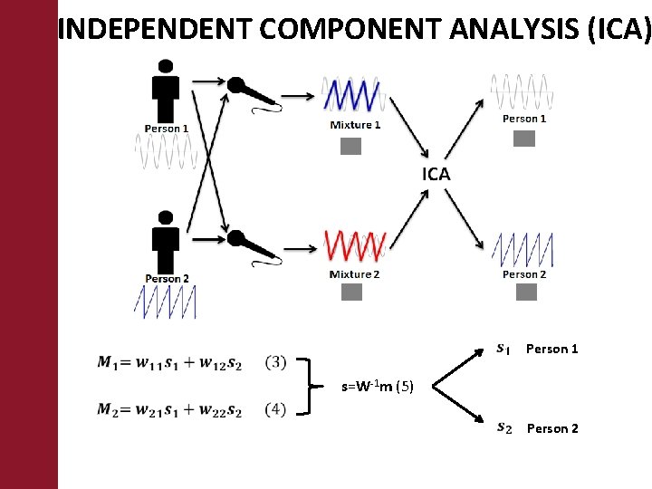
INDEPENDENT COMPONENT ANALYSIS (ICA) Person 1 s=W-1 m (5) Person 2

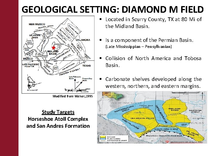
GEOLOGICAL SETTING: DIAMOND M FIELD § Located in Scurry County, TX at 80 Mi of the Midland Basin. § Is a component of the Permian Basin. (Late Mississippian – Pensyllvanian) § Collision of North America and Tobosa Basin. § Carbonate shelves developed along the western, northern, and eastern margins. Modified from Walker, 1995 Study Targets Horseshoe Atoll Complex and San Andres Formation

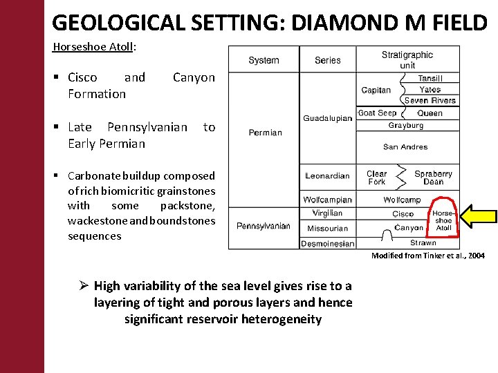
GEOLOGICAL SETTING: DIAMOND M FIELD Horseshoe Atoll: § Cisco and Formation Canyon § Late Pennsylvanian Early Permian to § Carbonate buildup composed of rich biomicritic grainstones with some packstone, wackestone and boundstones sequences Modified from Tinker et al. , 2004 Ø High variability of the sea level gives rise to a layering of tight and porous layers and hence significant reservoir heterogeneity

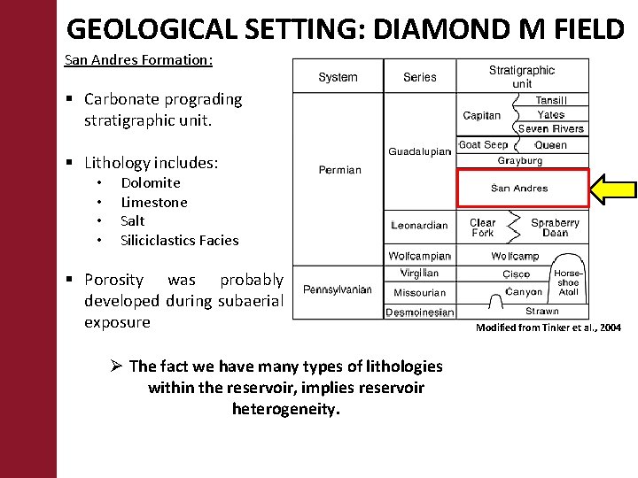
GEOLOGICAL SETTING: DIAMOND M FIELD San Andres Formation: § Carbonate prograding stratigraphic unit. § Lithology includes: • • Dolomite Limestone Salt Siliciclastics Facies § Porosity was probably developed during subaerial exposure Ø The fact we have many types of lithologies within the reservoir, implies reservoir heterogeneity. Modified from Tinker et al. , 2004

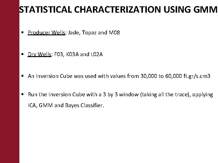
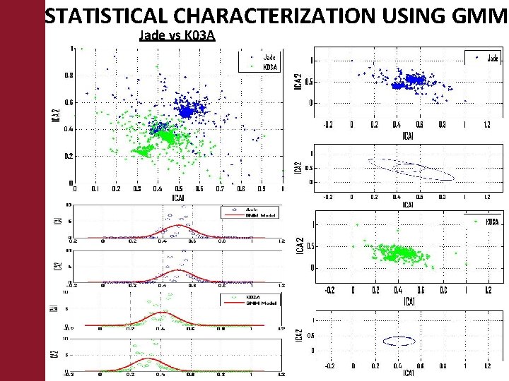
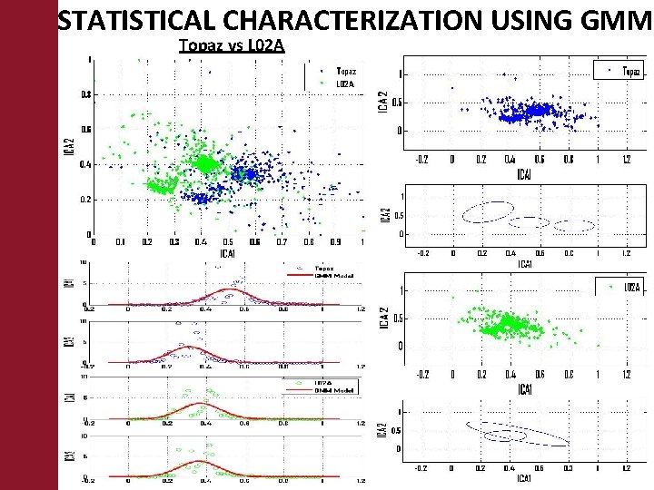
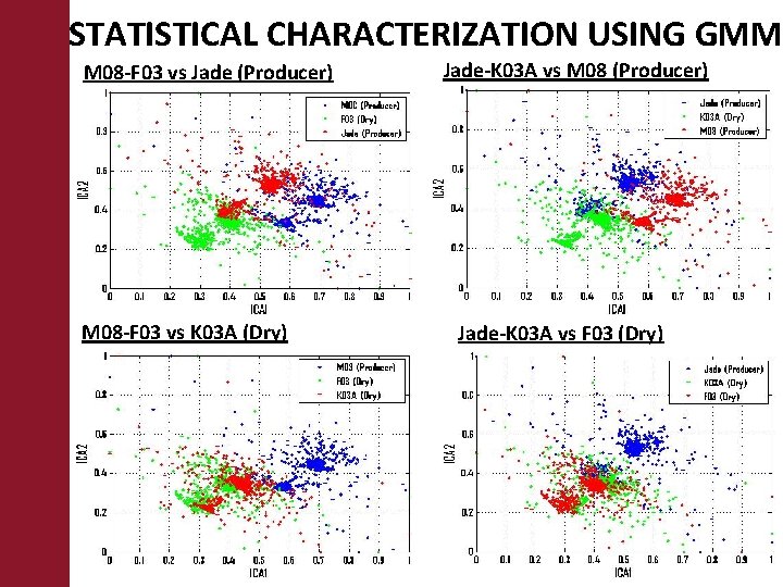
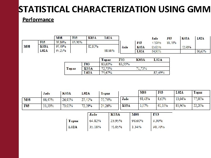
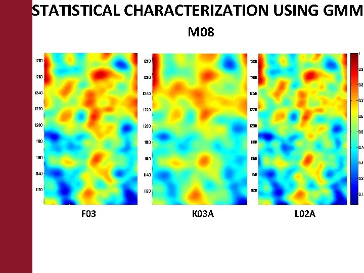
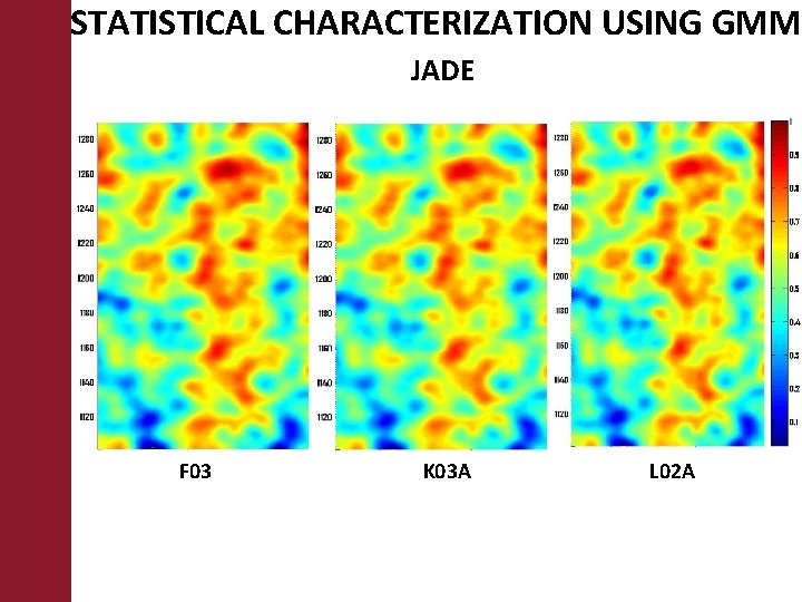
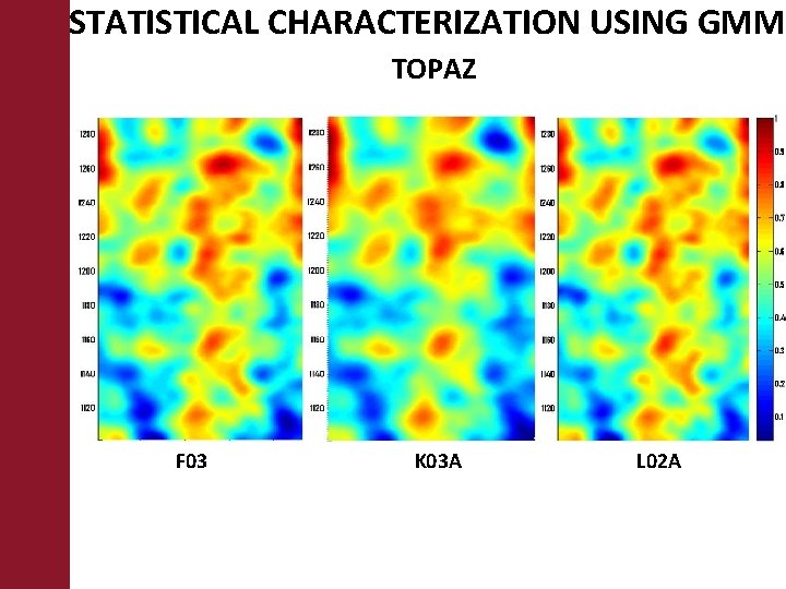
STATISTICAL CHARACTERIZATION USING GMM § Producer Wells: Jade, Topaz and M 08 § Dry Wells: F 03, K 03 A and L 02 A § An Inversion Cube was used with values from 30, 000 to 60, 000 ft. gr/s. cm 3 § Run the Inversion Cube with a 3 by 3 window (taking all the trace), applying ICA, GMM and Bayes Classifier.

STATISTICAL CHARACTERIZATION USING GMM

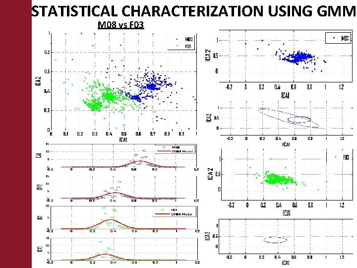
STATISTICAL CHARACTERIZATION USING GMM M 08 vs F 03

STATISTICAL CHARACTERIZATION USING GMM Jade vs K 03 A

STATISTICAL CHARACTERIZATION USING GMM Topaz vs L 02 A

STATISTICAL CHARACTERIZATION USING GMM M 08 -F 03 vs Jade (Producer) M 08 -F 03 vs K 03 A (Dry) Jade-K 03 A vs M 08 (Producer) Jade-K 03 A vs F 03 (Dry)

STATISTICAL CHARACTERIZATION USING GMM Performance

STATISTICAL CHARACTERIZATION USING GMM M 08 F 03 K 03 A L 02 A

STATISTICAL CHARACTERIZATION USING GMM JADE F 03 K 03 A L 02 A

STATISTICAL CHARACTERIZATION USING GMM TOPAZ F 03 K 03 A L 02 A

CONCLUSIONS § We propose a workflow based on independent component analysis and Gaussian mixture models that statistically represent the variability measured between the producers and dry wells. This characterization is derived without any user intervention. For this reason, it is called an “automatic learning” GMM. § The variability in Gaussian Mixture Model (GMM) represents the lateral and vertical changes seen in acoustic impedance within the reservoir. Although making probability maps, using the variability between wells, allow us to identify and quantify possible sweet-spots. § In a situation when we have thousands of wells in a resource play, the propose workflow can determine which wells are alike and which are different. We can also deduce if is there a correlation to those that are alike or different to know where we have good EUR. § The algorithm is really fast, each map can be made in 30 minutes using a personal computer.

ACKNOWLEDGEMENTS We thank to Parallel Petroleum LLC for the use of their data and the Attribute -Assisted Seismic Processing and Interpretation (AASPI) consortium for its financial support. Graphics were made using licenses to Petrel, provided to OU for research and education courtesy of Schlumberger.

QUESTIONS